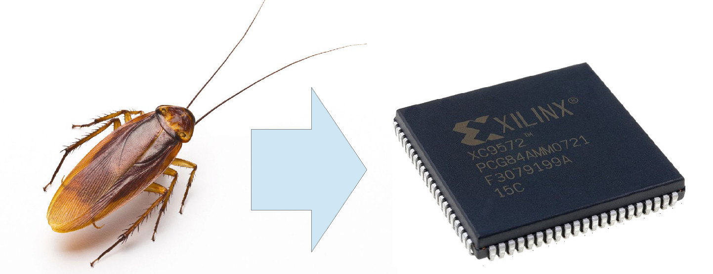
With the development of the Bug trap and press (Link) (Link) the down trodden Bugs have taken up arms and developed a fleet of robo-cockroaches. Ive tried to help them by developing a bio-inspired cockroach. The aim of this project is to show how a set of simple finite state machines can be designed, implemented in hardware, then used to produce a robot that has cockroach like tendencies. During the first year of the undergraduate program students are taught the mathematical theory of state machines and how to implement these in hardware. However, the ideas presented during these two modules can sometimes seem detached i.e. state diagrams, mathematical proofs and software implementations (applications), verses Boolean logic gates and flip-flops. This work looks at how these design techniques (representations) can be applied to a slightly more complex system, hopefully making links between these differing faces of the finite state machine. So how do you implement a cockroach in hardware?
Obstacle Avoidance
Loop Detector
Random movement
Blocked-in detector
Explore
Prototype 1
Seek Darkness
Follow Walls
Eat food
Figure 1 : cockroach into a complex programmable logic device (CPLD)

Figure 2 :
Trying to define the essence of a cockroach is a bit tricky. My first attempt is shown in the state diagram, figure 3. I'm sure there are better / alternative behaviours. The three core behaviours where:
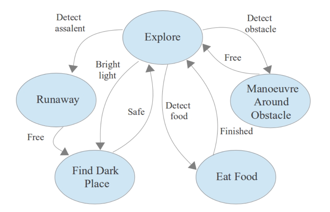
Figure 3 : Top level behaviour
As this cockroach is an electrical beast, food will be a recharging point, but otherwise the final robot should exhibit the same sorts of responses you would expect to see from a normal cockroach. A behaviour control network will be used to implement the cockroach's brain. Sometimes called a Subsumption architecture (Link), this approach was suggested by R. Brookes as an alternative solution to the traditional world modelling / planning robot control paradigm. These controllers define a series of behaviours, each behaviour working in parallel, converting sensor inputs into actuator control signals. Behaviours are given a priorities, higher level behaviours can temporarily suppress lower level behaviours i.e. subsume their behaviour, as shown in figure 4. I've partitioned the cockroach's behaviour into two networks: explore and find food. Sensors are listed on the left, actuators on on the right. Within each network low level behaviours are at the bottom, high level behaviours are at the top. Suppression points are indicated by circles, labelled with an 'S'. The important point to remember is that each behaviour is implemented as a state machine. All state machines are running in parallel. When a higher level behaviour becomes active it does not stop lower level behaviours, it only suppresses its output, replacing it with its own. Notes, the cockroaches behaviour could of been defined in a number of different ways, i went for this two component split to simplify construction and testing (i.e. just in case i needed to split the hardware over multiple devices).
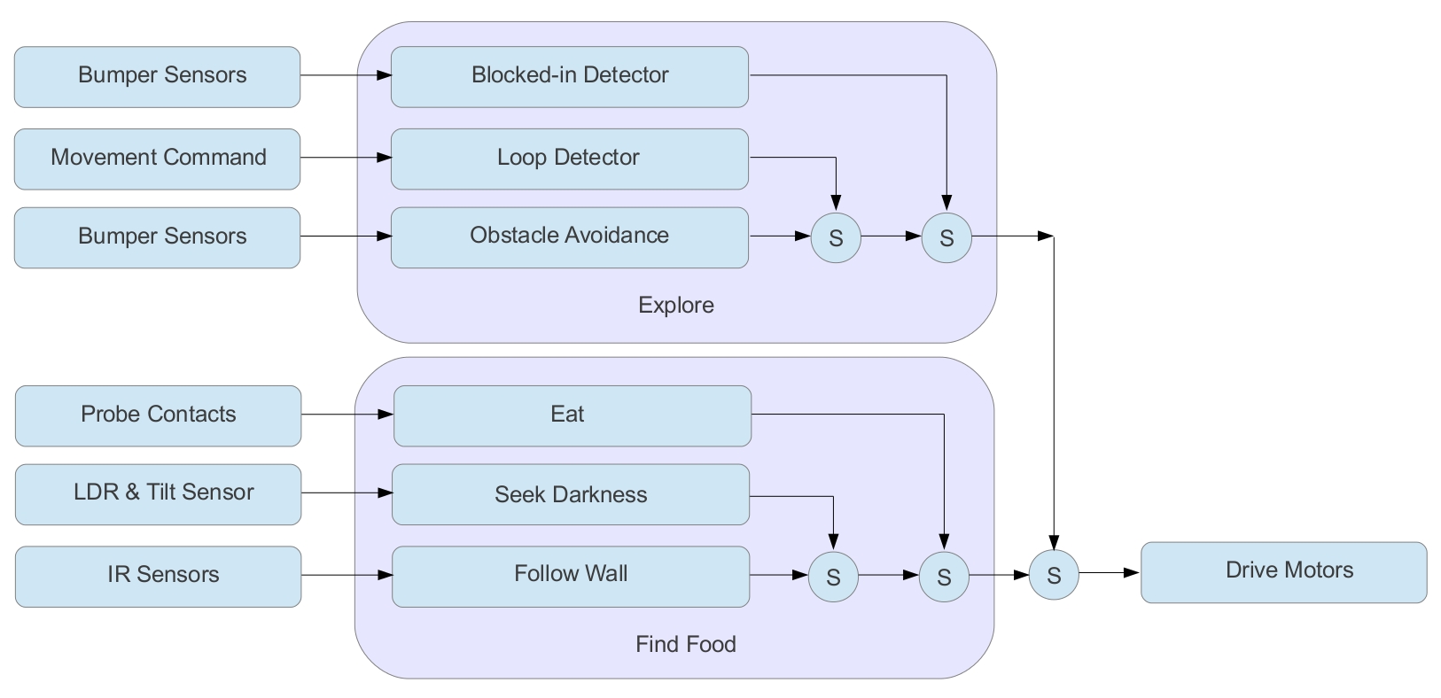
Figure 4 : Subsumption architecture
Behaviour based control tightly couples sensor data to actuator actions i.e. a behaviour can be thought of as a simple reflex. This minimises processing, allowing the robot to respond very quickly to changes in its environment. Complex behaviours are created through the interaction of these simple behaviours i.e. suppression points. This method of defining a robot's behaviour allows an incremental development, new layers of behaviours can be added to the system without having to modify lower levels. Therefore, the key to this technique are sensors, these systems do not have a world view (a map, knowledge of its environment it is moving through), all actions must be based on input sensor data. For this robot these will be:
The base behaviour for the explore network is obstacle avoidance. This is based on the front and rear bumper whisker sensors. The cockroaches behaviour is based on exploring a maze type environment. Simple connected mazes, shown in figure 6, can be explored using the left hand rule, following the outer wall (Link). More complex mazes with free standing wall elements are more difficult to solve, needing additional behaviours e.g. looping detection, following a free standing wall element, blocked-in detection, trapped between two wall elements. Note, this robot will be implemented using very minimal hardware, very limited memory, therefore optimal solutions will not be possible.
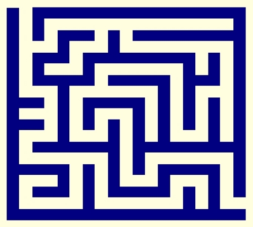
Figure 5 : Environment: connected maze

Figure 6 : Environment: complex maze
The default behaviour of the robot to explore the maze is to move forwards, if the whiskers detect a wall it will move backwards into free space so that is can turn (should be free as the robot has just travelled through this area), turn 90 degree, such that it is facing away from the obstacle, then continue forwards, as shown in figure 7. The state machine to implement these control signals is shown in figure 8. Each state is shown as an oval, the SX number above the line is the state identifier, the names and values below the lines are the outputs for that state. Names on connecting arcs define the condition that must be true for that state to be entered. If there is no condition on a arc, the transition is unconditional i.e. the state machine automatically moves to that state on the next time interval.
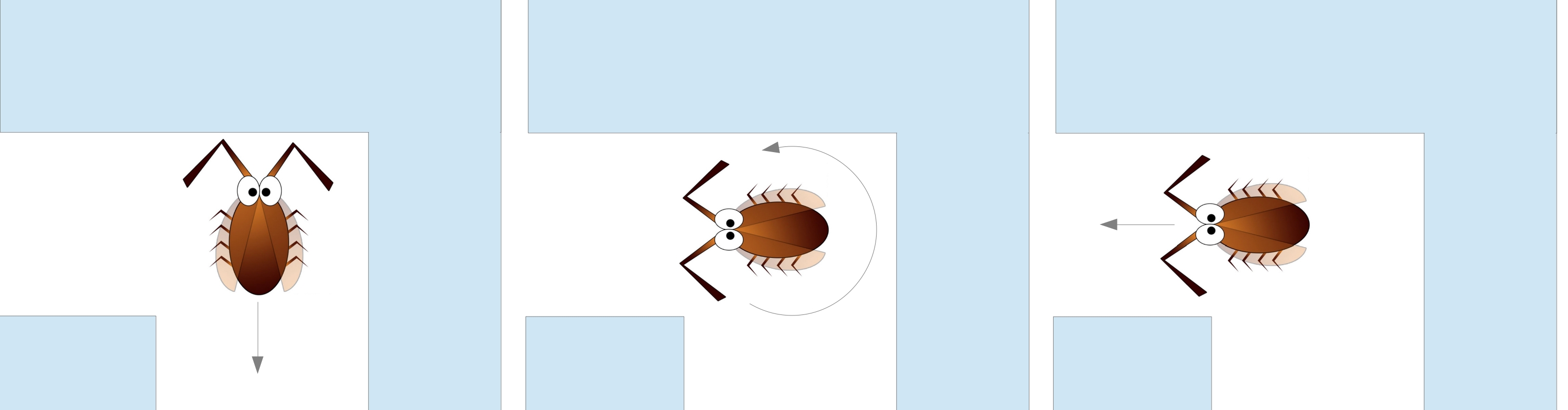
Figure 7 : Obstacle avoidance movements
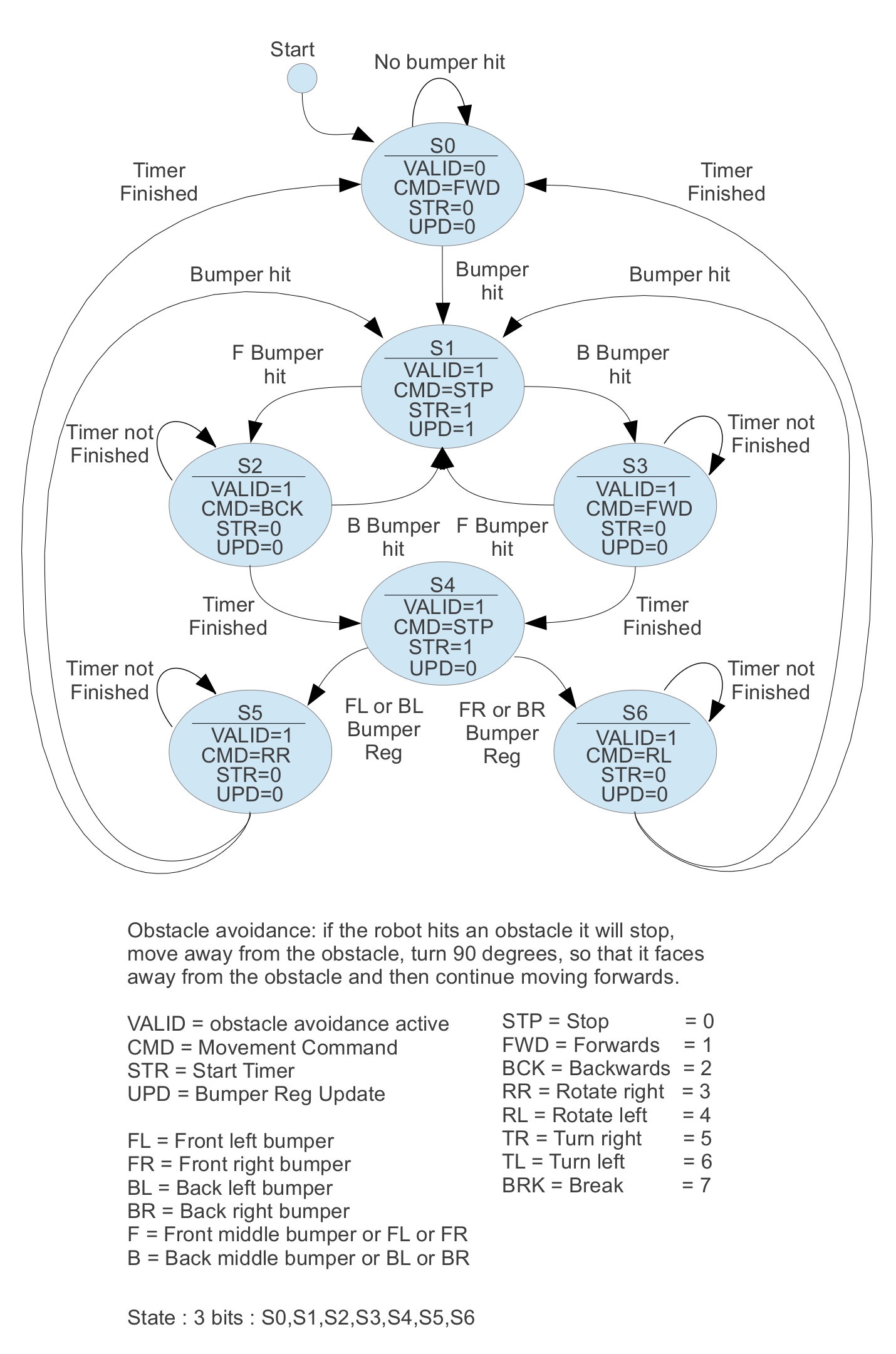
Figure 8 : Obstacle avoidance state diagram
Whisker data is 'pre-processed' through a logic circuit (described later), to produce the input signals Bumper-hit, F bumper, B bumper etc. The robot uses simple open loop motor control, knowing the average motor speed, distances or angles are measured using a timer (555 timer described later) e.g. moving forwards for 2 seconds the robot will travel approximately 15cm, or rotating for 2 seconds the robot will turn approximately 90 degrees. Ideally sensors mounted on the wheels or drive motors would be used to measure these distances, however, this would of required additional hardware, perhaps for version 2. The main output from this state machine is the motor command (CMD), this is a 3bit value defining seven possible movements. Note, rotate is when both motor are on, rotating in different directions, robot rotates about its drive axis. Turing is when one motor is on and the other is stopped i.e. brake, robot rotates about the stopped wheel. This 3bit code is sent to the motor drive logic which decodes it into the required control signals.
The state machines used in the Subsumption architecture are implemented in a Complex Programmable Logic Device (CPLD) (Link) (Link). As discussed in Lectures a state machine is implemented from three blocks: input forming logic (IFL), output forming logic (OFL) and a state register, as shown in figure 9. The mapping of state identifier to binary code is shown in figure 10. The input forming logic truth table, defining the relationship between input signals and the present state PS2:PS1:PS0 to the next state NS2:NS1:NS0 is shown in figure 11. The state machines used are Moore state machines (Link), therefore, outputs are only based on the present state, as shown in figure 12.
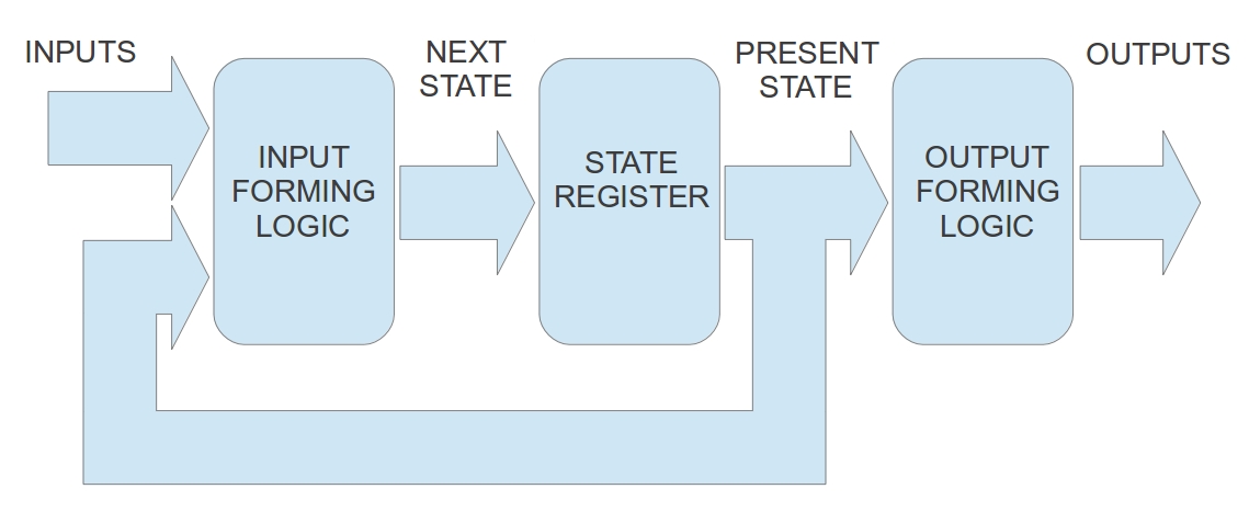
Figure 9 : State machine.
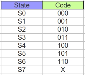
Figure 10 : Obstacle avoidance state encoding.
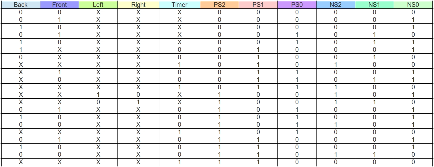
Figure 11 : Obstacle avoidance input forming logic.
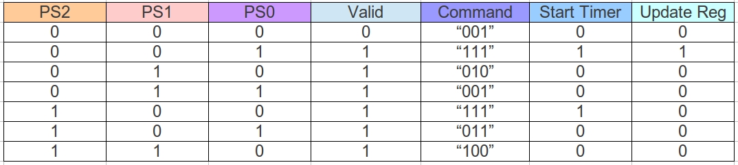
Figure 12 : Obstacle avoidance output forming logic.
Converting these truth tables into Boolean logic equations can be done using the laws of Boolean algebra, or Karnaugh Maps (Kmaps). The easiest method is Kmaps, but these are limited to 2, 3, 4 or 5 input variables. Therefore, owing to the large number of inputs you are normally limited to Boolean algebra for the input forming logic, however, Karnaugh Maps can be used for the output forming logic. The sum of products (SOP) representation for the input forming logic are shown below. Don't care inputs (X) can be ignored, terms that are common across multiple outputs can be shared i.e. to minimise gate count.
B   F   L   R   T   P2  P1  P0            TERMS
X   X   X   X   1   0   1   0       T & !P2 &  P1 & !P0
X   X   X   X   1   0   1   1       T & !P2 &  P1 &  P1
X   X   1   0   X   1   0   0       L & !R  &  P2 & !P1 & !P0          SHARE1
X   X   0   1   X   1   0   0      !L &  R  &  P2 & !P1 & !P0          SHARE2
0   0   X   X   0   1   0   1      !B & !F  & !T  &  P2 & !P1 & P0     SHARE3
0   0   X   X   0   1   1   0      !B & !F  & !T  &  P2 &  P1 & P0     SHARE4

SHARE1 =  L & !R  &  P2 & !P1 & !P0
SHARE2 = !L &  R  &  P2 & !P1 & !P0
SHARE3 = !B & !F  & !T  &  P2 & !P1 & P0
SHARE4 = !B & !F  & !T  &  P2 &  P1 & P0

NS2    = (T & !P2 & P1 & !P0) + (T & !P2 & P1 & P1) +
         SHARE1 + SHARE2 + SHARE3 + SHARE4

B   F   L   R   T   P2  P1  P0            TERMS
0   1   X   X   X   0   0   1      !B &  F  & !P2 & !P1 & P0
1   0   X   X   X   0   0   1       B & !F  & !P2 & !P1 & P0           SHARE5
0   0   X   X   0   0   1   0      !B & !F  & !T  & !P2 &  P1 & !P0
0   0   X   X   0   0   1   1      !B & !F  & !T  & !P2 &  P1 &  P0    SHARE6
X   X   0   1   X   1   0   0      !L &  R  &  P2 & !P1 & !P0          SHARE2
0   0   X   X   0   1   1   0      !B & !F  & !T &  P2 &  P1 & !P0     SHARE4

SHARE5 =  B & !F  & !P2 & !P1 & P0
SHARE6 = !B & !F  & !T  & !P2 & P1 &  P0

NS1    = (!B & F & !P2 & !P1 & P0) + (!B & !F & !T & !P2 & P1 & !P0) +
         SHARE2 + SHARE4 + SHARE5 + SHARE6

B   F   L   R   T   P2  P1  P0            TERMS
0   1   X   X   X   0   0   0      !B &  F & !P2 & !P1 & !P0
1   0   X   X   X   0   0   0       B & !F & !P2 & !P1 & !P0
1   0   X   X   X   0   0   1       B & !F & !P2 & !P1 &  P0           SHARE5
1   X   X   X   0   0   1   0       B & !T & !P2 &  P1 & !P0
X   1   X   X   0   0   1   1       F & !T & !P2 &  P1 &  P0
0   0   X   X   0   0   1   1      !B & !F & !T  & !P2 &  P1 &  P0     SHARE6
X   X   1   0   X   1   0   0       L & !R &  P2 & !P1 & !P0           SHARE1
0   1   X   X   0   1   0   1      !B &  F & !T  &  P2 & !P1 &  P0
1   0   X   X   0   1   0   1       B & !F & !T  &  P2 & !P1 &  P0
0   0   X   X   0   1   0   1      !B & !F & !T  &  P2 & !P1 &  P0     SHARE3
0   1   X   X   0   1   1   0      !B &  F & !T  &  P2 &  P1 & !P0
1   0   X   X   0   1   1   0       B & !F & !T  &  P2 &  P1 & !P0

NS0 = (!B & F & !P2 & !P1 & !P0) + (B & !P2 & !P1 & !P0) + (B & !F & !T  & !P2 & P1 & !P0) +
      (F & !T & !P2 & P1 & P0) + (!B &  F & !T & P2 & !P1 & P0) + (B & !F & !T & P2 & !P1 & P0) +
      (!B & F & !T & P2 & P1 & !P0) + (B & !F & !T & P2 & P1 & !P0) + SHARE1 + SHARE3 + SHARE5 + SHARE6
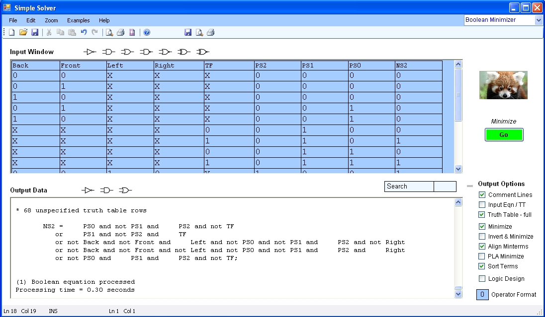
Figure 13 : Simple Solver minimisation
However, being lazy i cut-and-pasted these truth tables from the original spread sheet into Simple Solver (Link), shown in figure 13. The first eight columns are inputs, the final column is the output, column labels must not use ' ', '-', '_' and tables must end with a ';' character. This application produced the minimised equations below:
NS2 <=            (Left and not PS0   and not PS1 and     PS2 and not Right)
           or     (PS1  and not PS2   and     Timer)
           or (not Back and not Front and     PS0 and not PS1 and     PS2 and not Timer)
           or (not Back and not Front and not PS0 and     PS1 and     PS2 and not Timer)
           or (not Left and not PS0   and not PS1 and     PS2 and     Right);

NS1 <=            (Back  and not Front and     PS0 and not PS1 and not PS2)
           or (not Back  and     Front and     PS0 and not PS1 and not PS2)
           or (not Back  and not Front and not PS0 and     PS1 and not Timer)
           or (not Back  and not PS0   and     PS1 and not PS2 and not Timer)
           or (not Front and     PS0   and     PS1 and not PS2 and not Timer)
           or (not Left  and not PS0   and not PS1 and     PS2 and     Right);

NS0 <=            (Back  and     PS1   and not PS2 and not Timer)
           or     (Back  and not Front and not PS0 and     PS1 and not Timer)
           or     (Back  and not Front and not PS1 and not PS2)
           or     (Left  and not PS0   and not PS1 and     PS2 and not Right)
           or     (PS0   and     PS1   and not PS2 and not Timer)
           or (not Back  and     Front and not PS0 and     PS1 and     PS2 and not Timer)
           or (not Back  and     Front and not PS0 and not PS1 and not PS2)
           or (not Back  and     PS0   and not PS1 and     PS2 and not Timer)
           or (not Front and     PS0   and not PS1 and     PS2 and not Timer);
Figure 14 : VHDL - obstacle avoidance input forming logic (IFL).
These auto-generated equations may not be the best solution, as a human can optimise the truth tables e.g. add / remove don't care states, combine terms, change encodings, modify the design for the particular CPLD architecture used etc. However, its quick and does remove human error. Output performing logic can be minimised using Karnaugh Maps, as shown below:
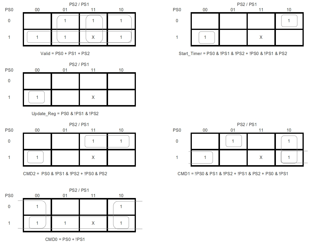
Figure 15 : Obstacle avoidance output forming logic.
Simple Solver produced the minimised equations below, not quite as small as Kmaps which use a don't care state i.e. the user has made the decision that state "111" will never be entered, therefore, that state can be defined as a 'Don't Care' (X). You could argue this is a dangerous assumption i.e. the robot could enter an unsafe state.
Valid <=        (PS0 and not PS1)
         or     (PS1 and not PS2)
         or (not PS0 and     PS2);

Start_Timer <=        (PS0 and not PS1 and not PS2)
               or (not PS0 and not PS1 and     PS2);

Update_Reg <= (PS0 and not PS1 and not PS2);

CMD2 <=        (PS0 and not PS1 and not PS2)
        or (not PS0 and     PS2);

CMD1 <=        (PS0 and not PS1)
        or (not PS0 and     PS1 and not PS2)
        or (not PS1 and     PS2);

CMD0 <=        (PS0 and not PS2)
        or (not PS1);
Figure 16 : VHDL - obstacle avoidance output forming logic (OFL).
Again to save time the IFL and OFL circuits can be defined as VHDL components as shown in the top level schematic in figure 17. The symbol FDC is a D-type flip-flop. The hardware requirements inside the CPLD are listed in figure 18. Initial hardware testing was performed using the simulation shown in figure 19.
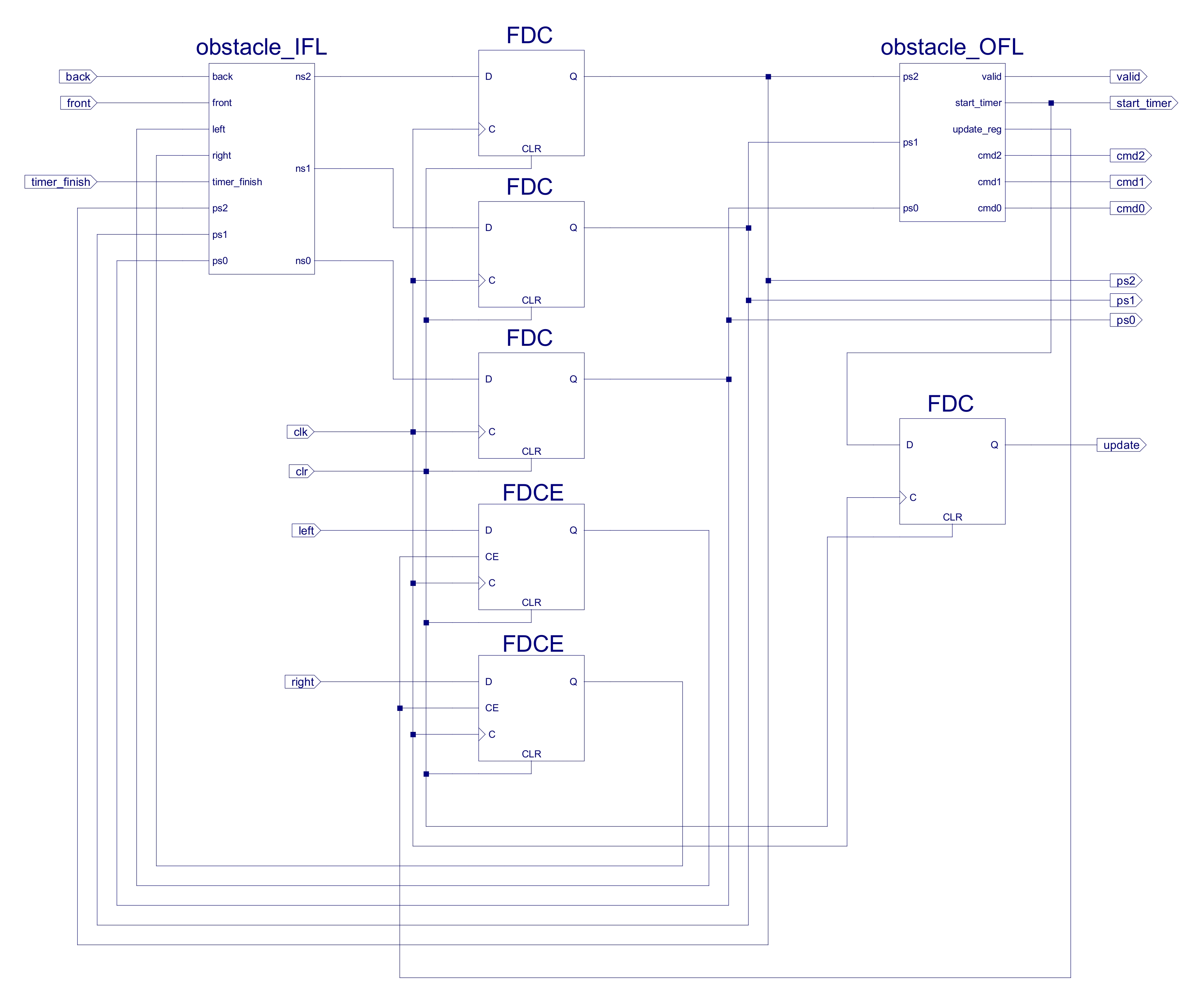
Figure 17 : Obstacle avoidance schematic.
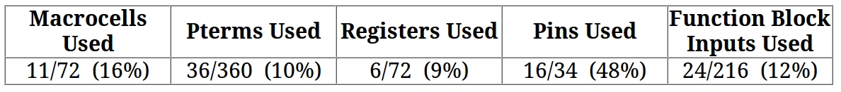
Figure 18 : Obstacle avoidance hardware requirements.
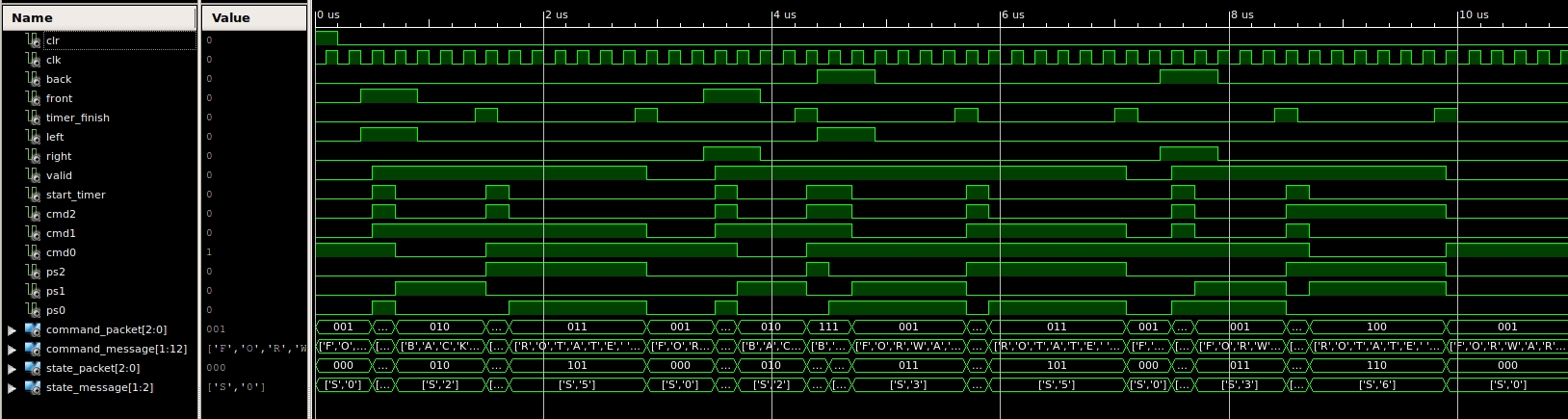
Figure 19 : Obstacle avoidance simulation.
In addition to manoeuvring around obstacles the robot also needs to detect if it is 'stuck'. This can take different forms, the first to be considered is looping. In mazes with free standing wall elements there is a danger that rather than exploring the maze the robot gets stuck circling a wall elements, as shown in figure 20. To detect this behaviour the state machine in figure 21 can be used.
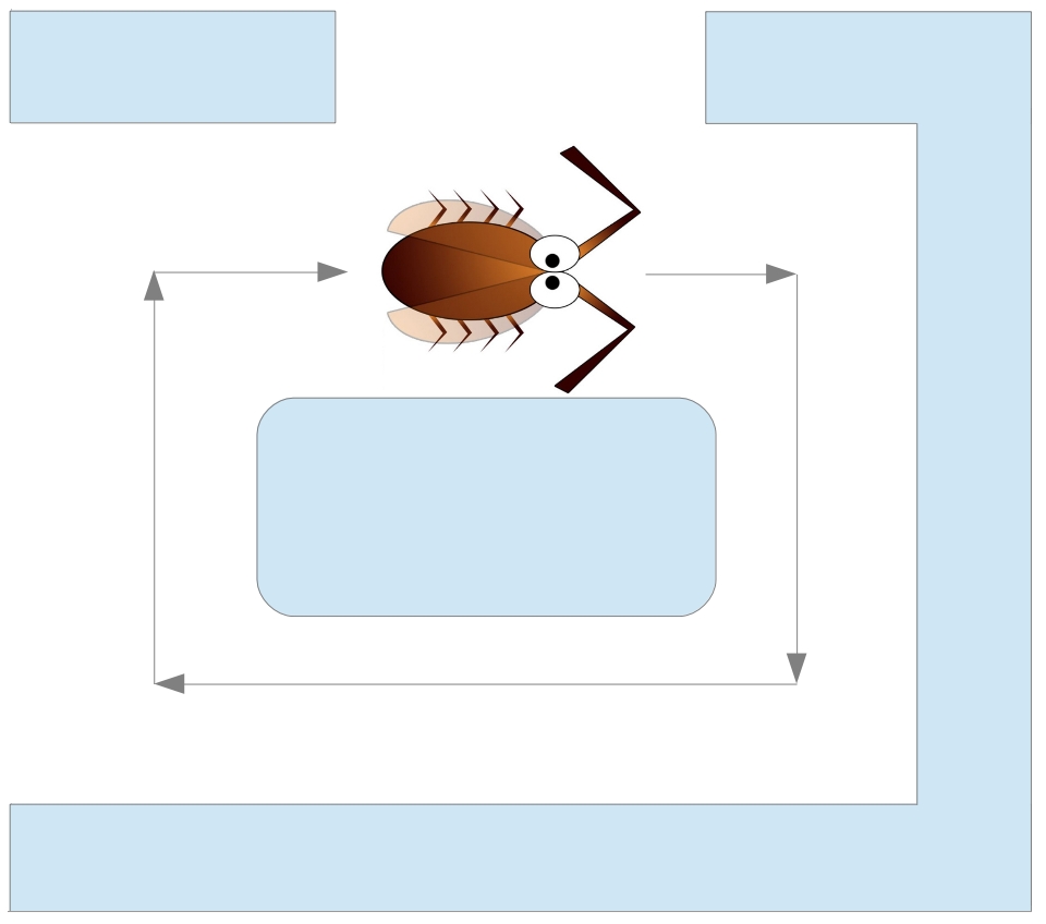
Figure 20 : Looping behaviour.
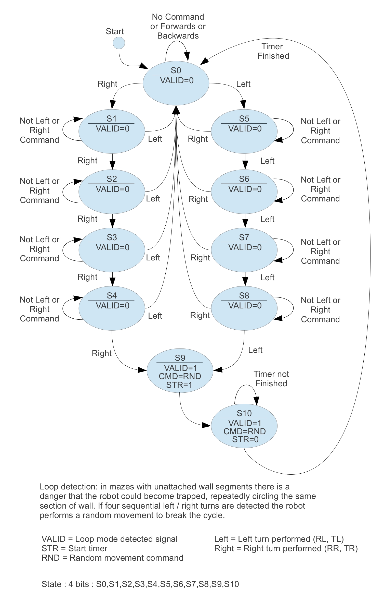
Figure 21 : Looping detection state machine.
Unlike the previous state machine this one is not directly driven by sensor data, rather it monitors the commands issued to the drive motors e.g. the UPDATE and CMD signals from the previous state machines (figure 17). If the state machine detects five sequential Left / Right turns it assumes it is 'stuck' and performs a random movement, hopefully pushing the robot into free space. Note, strictly speaking you only need to do four turns to loop, but decided add one more just to make sure. The mapping of state identifier to binary code is shown in figure 22. The input forming logic truth table, defining the relationship between input signals and the present state PS3:PS2:PS1:PS0 to the next state NS3:NS2:NS1:NS0 is shown in figure 23. The output forming logic truth table is shown in figure 24.
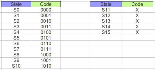
Figure 22 : Looping detector state encoding.
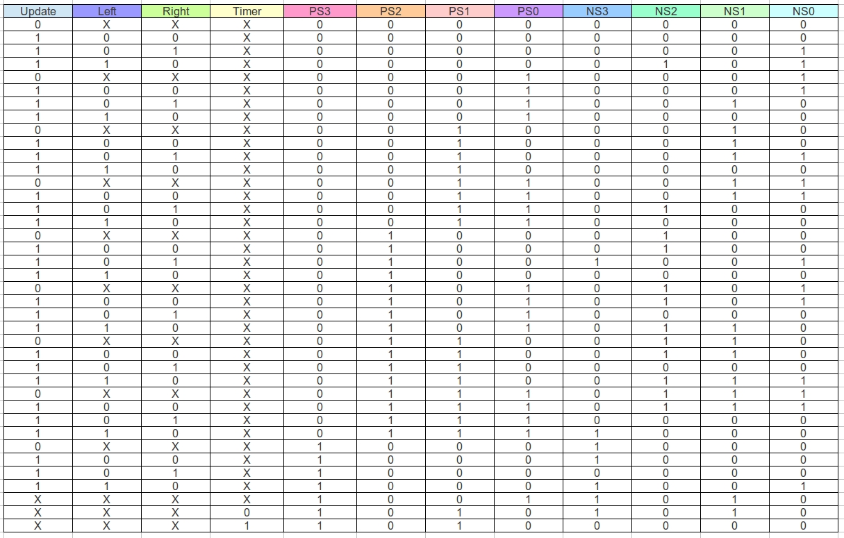
Figure 23 : Looping detector input forming logic.
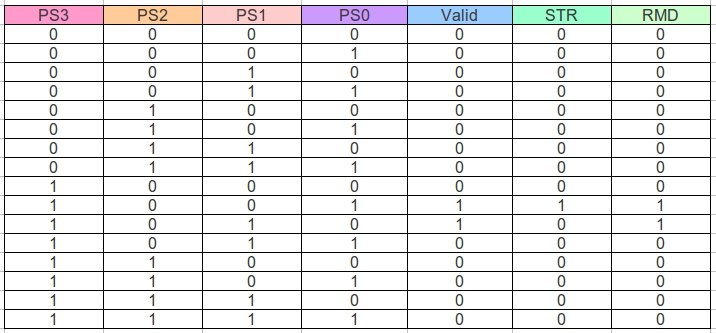
Figure 24 : Looping detector output forming logic.
Cut-and-pasting these into Simple Solver produced the following Boolean equations:
NS3 <=           (Left  and     PS0 and     PS1 and     PS2 and not PS3 and not Right and Update)
           or     (PS0  and not PS1 and not PS2 and     PS3
           or (not Left and not PS0 and not PS1 and     PS2 and not PS3 and     Right and Update)
           or (not PS0  and     PS1 and not PS2 and     PS3 and not Timer)
           or (not PS1  and not PS2 and     PS3 and not Right)
           or (not PS1  and not PS2 and     PS3 and not Update);

NS2 <=           (Left  and not PS0 and not PS1 and not PS2 and not PS3 and not Right and Update)
           or     (PS0  and not PS1 and     PS2 and not PS3 and not Right)
           or     (PS2  and not PS3 and not Update)
           or (not Left and     PS0 and     PS1 and not PS2 and not PS3 and     Right and Update)
           or (not Left and     PS2 and not PS3 and not Right)
           or (not PS0  and     PS1 and     PS2 and not PS3 and not Right);

NS1 <=           (Left  and     PS0 and not PS1 and     PS2 and not PS3 and not Right and Update)
           or     (PS0  and not PS1 and not PS2 and     PS3)
           or     (PS1  and not PS3 and not Update)
           or (not Left and     PS0 and not PS1 and not PS2 and     Right and   Update)
           or (not Left and     PS1 and not PS3 and not Right)
           or (not Left and not PS0 and     PS1 and not PS2 and not PS3)
           or (not PS0  and     PS1 and     PS2 and not PS3 and not Right)
           or (not PS0  and     PS1 and not PS2 and     PS3 and not Timer);

NS0 <=            (Left and not PS0 and     PS1 and     PS2 and not PS3 and not Right and Update)
           or     (Left and not PS0 and not PS1 and not PS2 and not Right and   Update)
           or     (PS0  and not PS3 and not Update)
           or (not Left and     PS0 and not PS3 and not Right)
           or (not Left and not PS0 and not PS1 and not PS3 and     Right and Update)
           or (not Left and not PS0 and not PS2 and not PS3 and     Right and Update);
Figure 25 : VHDL - loop detector input forming logic (IFL).
Valid <=         (PS0 and not PS1 and not PS2 and PS3)
          or (not PS0 and     PS1 and not PS2 and PS3);

STR   <=  (PS0 and not PS1 and not PS2 and PS3);

RMD   <=         (PS0 and not PS1 and not PS2 and PS3)
          or (not PS0 and     PS1 and not PS2 and PS3);
Figure 26 : VHDL - loop detector output forming logic (OFL).
Again to save time the IFL and OFL circuits can be defined as VHDL components as shown in the top level schematic in figure 27. The symbol FDCE is a D-type flip-flop with a clock enable (CE) pin. If CE=0, flip-flop will ignore CLK. If CE=1, flip-flop is updated on CLK rising edge. The hardware requirements inside the CPLD are listed in figure 28. Initial hardware testing was performed using the simulation shown in figure 29.
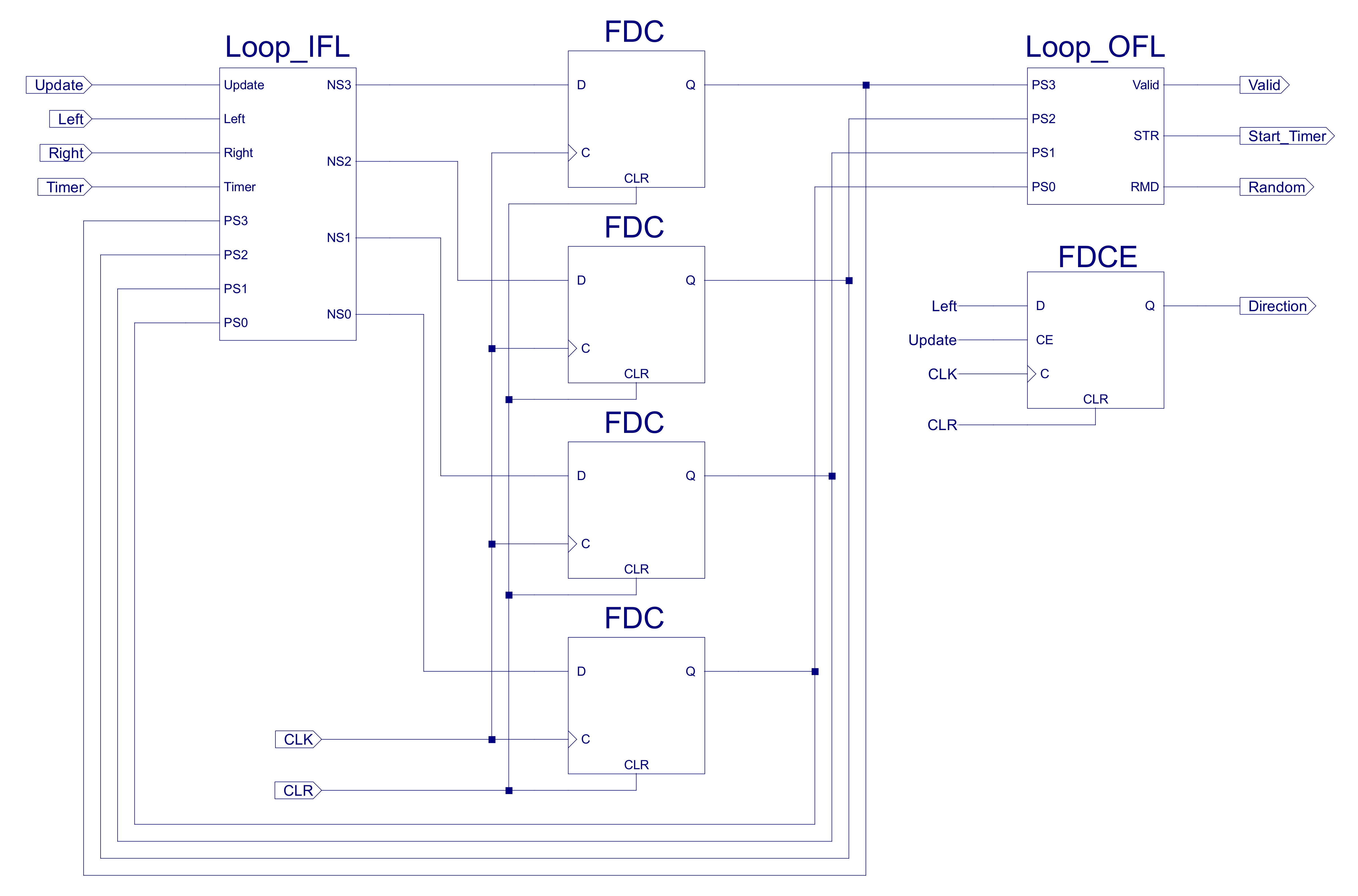
Figure 27 : Looping detector schematic.
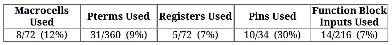
Figure 28 : Looping detector hardware requirements.
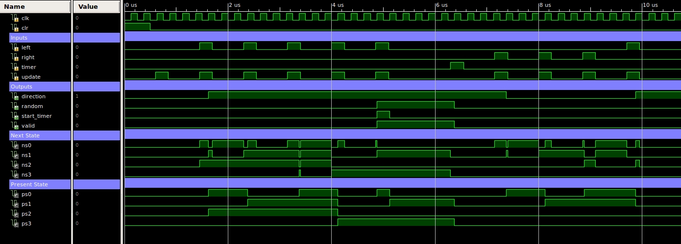
Figure 29 : Looping detector simulation.
To implement the random movement associated with states S9 and S10. The circuit shown in figure 30 is used. This is based on a Xilinx library component: CB2CE, a two bit binary counter with clock enable. This counter is free running i.e. on each rising clock edge the count is incremented, generating the output sequence: 0,1,2,3 and then back 0. Owing to the high speed of the clock signal compared to the robots movement the state of the counter will appear random when the Looping and Blocked-in (described later) behaviours are detected. This 'random' two bit state is combined with the Direction signal from the Loop detector in the output forming logic to produce a random command. This logic could be defined using truth tables as before, however, a quick method is to use the higher level VHDL construct: PROCESS. This allows you to define the logic's behaviour using IF-THEN-ELSE constructions as shown in figure 33. The Xilinx software tools then synthesise this description into a minimised logic circuit. If Looping behaviour is detected the robot will perform a turn in the opposite direction to the loop i.e. if the robot was always turning Left it will perform a Right turn, hopefully moving the robot into free space.
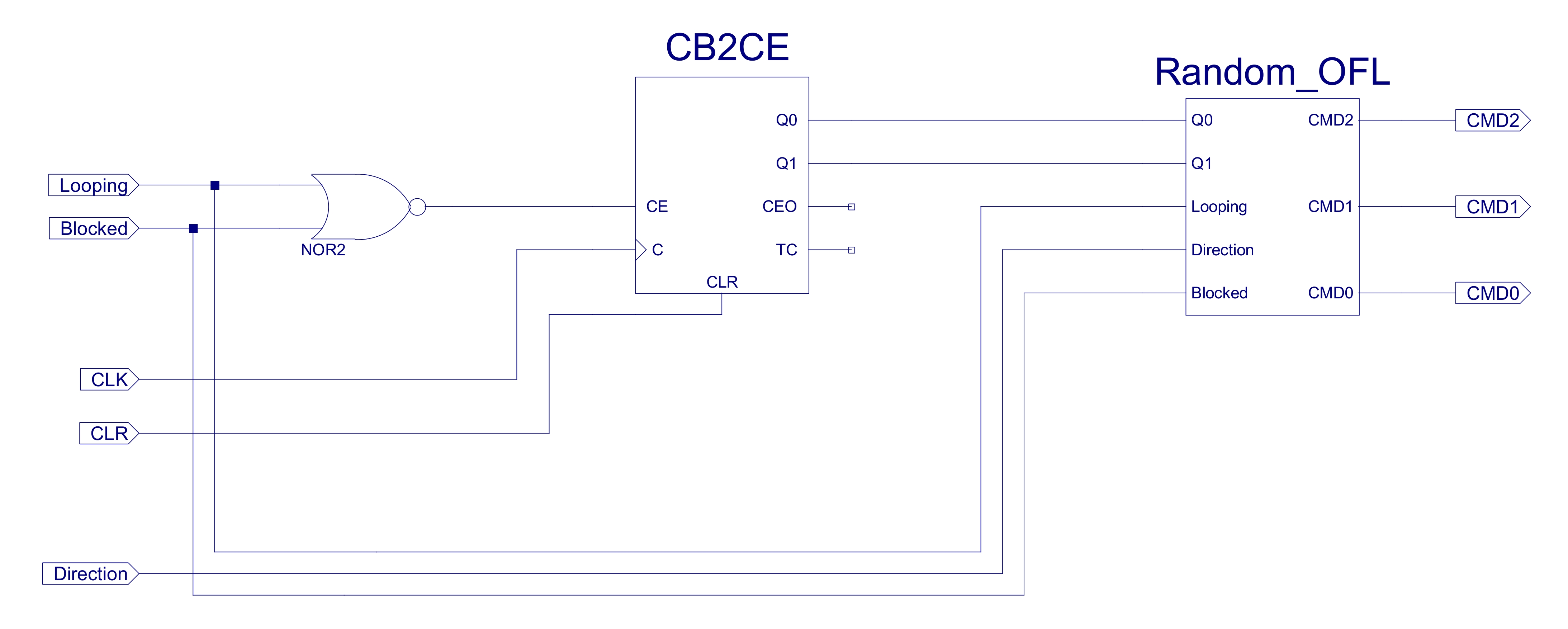
Figure 30 : Random command schematic.

Figure 31 : Random command hardware requirements.
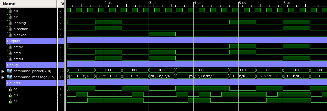
Figure 32 : Random command simulation.
library IEEE;
use IEEE.STD_LOGIC_1164.ALL;

entity Random_OFL is
    Port ( Q0 : in  STD_LOGIC;
           Q1 : in  STD_LOGIC;
           Looping : in  STD_LOGIC;
           Direction : in  STD_LOGIC;
           Blocked : in  STD_LOGIC;
           CMD2 : out  STD_LOGIC;
           CMD1 : out  STD_LOGIC;
           CMD0 : out  STD_LOGIC);
end Random_OFL;

architecture Random_OFL_arch of Random_OFL is

   constant STOP         : std_logic_vector(2 downto 0) := "000";
   constant FORWARDS     : std_logic_vector(2 downto 0) := "001";
   constant BACKWARDS    : std_logic_vector(2 downto 0) := "010";
   constant ROTATE_RIGHT : std_logic_vector(2 downto 0) := "011";
   constant ROTATE_LEFT  : std_logic_vector(2 downto 0) := "100";
   constant TURN_RIGHT   : std_logic_vector(2 downto 0) := "101";
   constant TURN_LEFT    : std_logic_vector(2 downto 0) := "110";
   constant BREAK        : std_logic_vector(2 downto 0) := "111";

   signal Count   : std_logic_vector(1 downto 0);
   signal Command : std_logic_vector(2 downto 0);

begin

   Count <= Q1 & Q0;
   CMD2  <= Command(2);
   CMD1  <= Command(1);
   CMD0  <= Command(0);

   logic: process( Count, Looping, Direction, Blocked )
   begin
      if Blocked='1'
      then
         case Count is
            when "00"   => Command <= ROTATE_RIGHT;
            when "01"   => Command <= TURN_RIGHT;
            when "10"   => Command <= ROTATE_LEFT;
            when "11"   => Command <= TURN_LEFT;
            when Others => Command <= STOP;
         end case;
      elsif Looping='1'
      then
         if Direction='1'
         then
            case Count is
               when "00"   => Command <= ROTATE_RIGHT;
               when "01"   => Command <= TURN_RIGHT;
               when "10"   => Command <= ROTATE_RIGHT;
               when "11"   => Command <= TURN_RIGHT;
               when Others => Command <= STOP;
            end case;
         else
            case Count is
               when "00"   => Command <= ROTATE_LEFT;
               when "01"   => Command <= TURN_LEFT;
               when "10"   => Command <= ROTATE_LEFT;
               when "11"   => Command <= TURN_LEFT;
               when Others => Command <= STOP;
            end case;
         end if;
      else
         Command <= STOP;
      end if;
   end process;

end Random_OFL_arch;
Figure 33 : VHDL - random command output forming logic (OFL).
The final behaviour in the explore component is Blocked-in. This is when the robot gets trapped between two wall elements, as shown in 34. Here the robot does not have enough room to complete the backwards movement defined in the Obstacle avoidance behaviour i.e. it will oscillate between states S1 and S2,S3. To prevent this behaviour the Blocked-in state machine counts the number of forwards-backwards movements performed in a sequence. If this exceeds a maximum threshold the robot performs a random movement to try and move into free space. Unlike the Looping detector state machine, the Blocked-in state machine uses an external counter i.e. a variable, rather than states to count these movements. This is based on a Xilinx library component: CB2LCE, a two bit binary counter with clock enable and parallel load. The L pin (load) is used to reset the counter i.e. load the value "00", the asynchronous CLR line could be used, however, this is not generally recommended as it can cause setup-and-hold timing problems within the CPLD. The maximum count threshold is trigger using the TC output from the counter. This produces a logical '1' when the the counter reaches the value "11".
Figure 34 : Blocked-in.
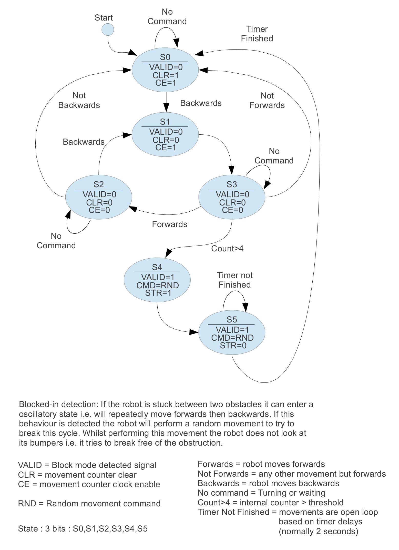
Figure 35 : Blocked-in state diagram.
The mapping of state identifier to binary code is shown in figure 36. The input forming logic truth table, defining the relationship between input signals and the present state PS2:PS1:PS0 to the next state NS2:NS1:NS0 is shown in figure 37. The output forming logic truth table is shown in figure 38.
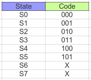
Figure 36 : Blocked-in state encoding.
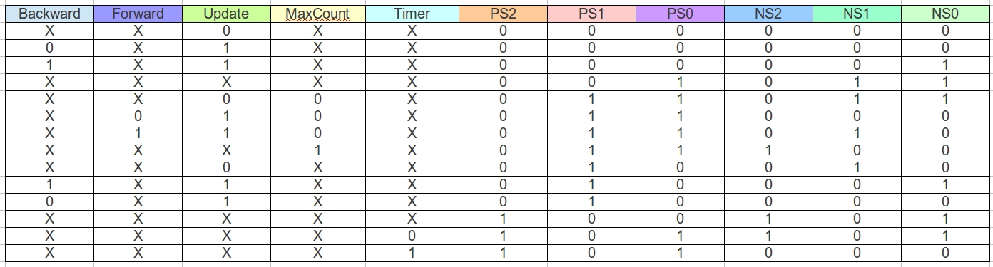
Figure 37 : Blocked-in input forming logic.
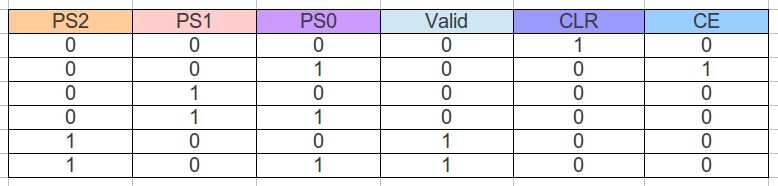
Figure 38 : Blocked-in output forming logic.
Cut-and-pasting these into Simple Solver produced the following Boolean equations:
NS2 <=        (Max_Count  and     PS0 and     PS1 and not PS2)
       or (not PS0        and not PS1 and     PS2)
       or (not PS1        and     PS2 and not Timer_Finish);

NS1 <=        (Forward   and not Max_Count and     PS0 and not PS2)
       or     (PS0       and not PS1       and not PS2)
       or (not Max_Count and     PS1       and not PS2 and not Update)
       or (not PS0       and     PS1       and not PS2 and not Update);

NS0 <=        (Backward  and not PS0 and not PS2 and     Update)
       or     (PS0       and not PS1 and not PS2)
       or (not Max_Count and     PS0 and not PS2 and not Update)
       or (not PS0       and not PS1 and     PS2)
       or (not PS1 and     PS2 and not Timer_Finish);
Figure 39 : VHDL - Blocked-in input forming logic (IFL).
valid       <= not PS1 and     PS2;
start_timer <= not PS0 and not PS1 and     PS2;
clr         <= not PS0 and not PS1 and not PS2;
ce          <=     PS0 and not PS1 and not PS2;
Figure 40 : VHDL - Blocked-in output forming logic (OFL).
Again to save time the IFL and OFL circuits can be defined as VHDL components as shown in the top level schematic in figure 41. The hardware requirements inside the CPLD are listed in figure 42. Initial hardware testing was performed using the simulation shown in figure 43.
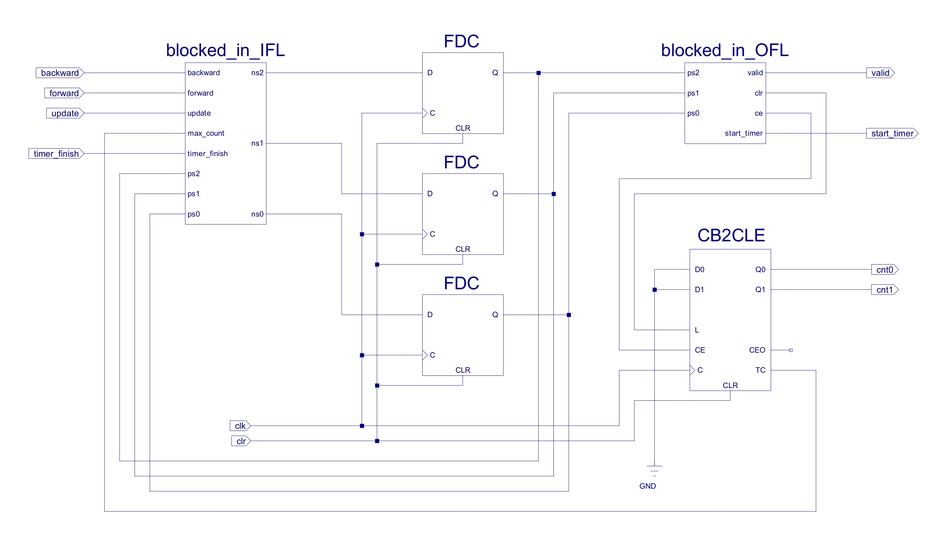
Figure 41 : Blocked-in schematic.

Figure 42 : Blocked-in hardware requirements.
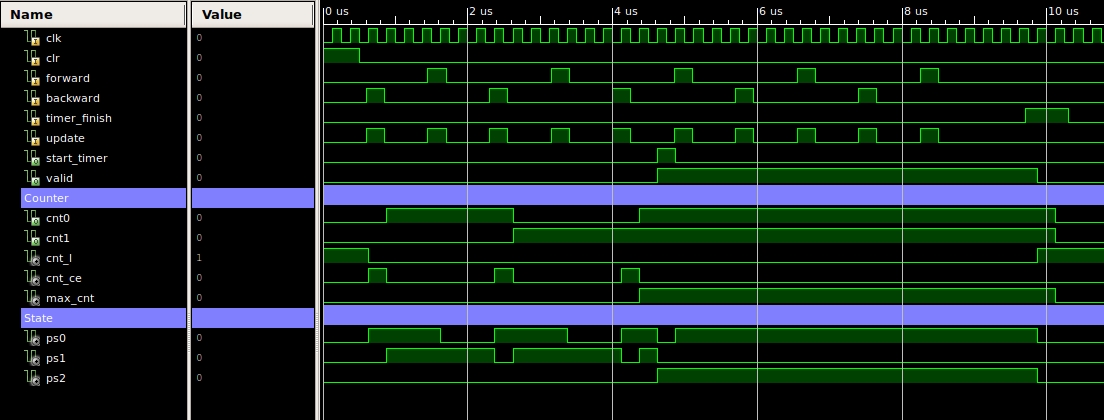
Figure 43 : Blocked-in simulation.
All three behaviours for the explore component are now complete, these are now integrated together to form the first Subsumption architecture, as shown in figure 44. The command used to control the drive motors can come from two sources: Obstacle avoidance, or random movement. Therefore, a multiplexer is required: mux_2_1_3. This 2:1, three bit multiplexer could be defined using a logic circuits, but to save time a VHDL description will be used, as shown in figure 45. If either the Looping detector or the Blocked-in behaviours are active the random movement generator is selected, it in turn is controlled by the VALID signals from these state machines.
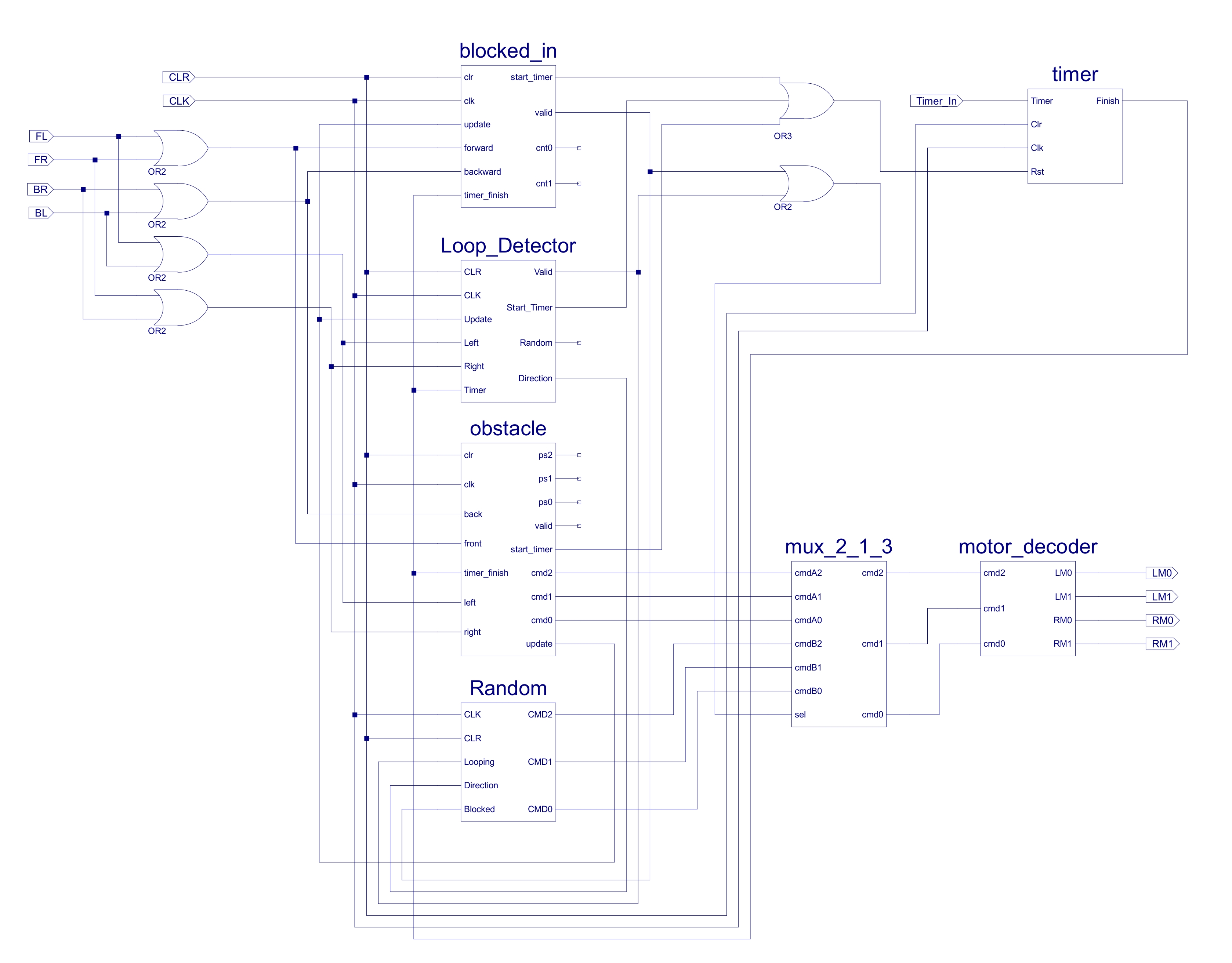
Figure 44 : Explore schematic.
library IEEE;
use IEEE.STD_LOGIC_1164.ALL;

entity mux_2_1_3 is
    Port ( cmdA2 : in  STD_LOGIC;
           cmdA1 : in  STD_LOGIC;
           cmdA0 : in  STD_LOGIC;
           cmdB2 : in  STD_LOGIC;
           cmdB1 : in  STD_LOGIC;
           cmdB0 : in  STD_LOGIC;
           cmd2  : out STD_LOGIC;
           cmd1  : out STD_LOGIC;
           cmd0  : out STD_LOGIC;
           sel : in  STD_LOGIC);
end mux_2_1_3;

architecture mux_2_1_3_arch of mux_2_1_3 is
begin

   mux: process( cmdA2, cmdA1, cmdA0, cmdB2, cmdB1, cmdB0, sel )
   begin
      if sel='0'
      then
         cmd2 <= cmdA2; cmd1 <= cmdA1; cmd0 <= cmdA0;
      else
         cmd2 <= cmdB2; cmd1 <= cmdB1; cmd0 <= cmdB0;
      end if;
   end process;

end mux_2_1_3_arch;
Figure 45 : VHDL - 2:1, 3bit multiplexer.
The output of this multiplexer is connected to the motor_decoder logic, converting the direction command codes into the required control signals for the two motor controller ICs: bd621x-e (Link), left motor control signals LM1:LM0, right motor control signals RM1:RM0. The robot has two drive motors and is manoeuvred using differential steering e.g. if both motors turn in the same direction the robot will move in a 'straight' line, if they turn in different directions the robot will rotate. The logic to implement this decoder is defined by the VHDL below:
library IEEE;
use IEEE.STD_LOGIC_1164.ALL;

entity motor_decoder is
    Port ( cmd2 : in  STD_LOGIC;
           cmd1 : in  STD_LOGIC;
           cmd0 : in  STD_LOGIC;
           LM0  : out STD_LOGIC;
           LM1  : out STD_LOGIC;
           RM0  : out STD_LOGIC;
           RM1  : out STD_LOGIC);
end motor_decoder;

architecture motor_decoder_arch of motor_decoder is

   signal command : std_logic_vector(2 downto 0);

begin

   command <= cmd2 & cmd1 & cmd0;

   logic : process( command )
   begin
      case command is
         when "000"  => LM1 <= '0'; LM0 <= '0'; RM1 <= '0'; RM0 <= '0'; --stop
         when "001"  => LM1 <= '0'; LM0 <= '1'; RM1 <= '0'; RM0 <= '1'; --forward
         when "010"  => LM1 <= '1'; LM0 <= '0'; RM1 <= '1'; RM0 <= '0'; --backward
         when "011"  => LM1 <= '1'; LM0 <= '0'; RM1 <= '0'; RM0 <= '1'; --rotate right
         when "100"  => LM1 <= '0'; LM0 <= '1'; RM1 <= '1'; RM0 <= '0'; --rotate left
         when "101"  => LM1 <= '0'; LM0 <= '1'; RM1 <= '0'; RM0 <= '0'; --turn right
         when "110"  => LM1 <= '0'; LM0 <= '0'; RM1 <= '0'; RM0 <= '1'; --turn left
         when "111"  => LM1 <= '1'; LM0 <= '1'; RM1 <= '1'; RM0 <= '1'; --brake
         when others => LM1 <= '0'; LM0 <= '0'; RM1 <= '0'; RM0 <= '0'; --stop
      end case;
   end process;

end motor_decoder_arch;
Figure 46 : VHDL - motor controller
Motor control is open loop (Link), distances and rotations are not measured, but are controlled by a timer i.e. drive motor speed is fixed, therefore, on a level, smooth surface, with a constant supply voltage the distance moved by each motor is proportional to time. These time delays are significantly longer than the system clock period, therefore, a 555 timer is used to generate a slower 'clock', in this example 128Hz, shown in figure 47. The 555 timer's output is connected to the Timer input of the edge detector circuit shown in figure 48. This circuit contains a two stage shift register, storing the present Timer signal and its previous value, updated using the system clock i.e. every 250ns (4MHz). If the Timer signal does not change these two samples will be the same, the AND gate (with one inverted input) will therefore output a logic '0'. If there is a 0->1 transition on the 555 timer output, shift register's state will be "10" which will cause the AND gate to produce a logic '1', for one clock cycle. This pulse is used to increment the eight bit counter CB8CLE, when this reaches the value 255 the TC output pin will go high, signalling that the delay is complete i.e. 1/128 * 255 = 2 seconds. If during this period a higher level behaviour is triggered the time delay can be reset by pulsing the RST input. The hardware requirements for this system are listed in figure 49.
Note, for anyone that has played around with robots knows the above assumption that motor speed is constant is not correct, robots do not like to travel in straight lines, but for this robot we will assume it is true, to be honest a slight randomness in movement may help the robot explore its environment.
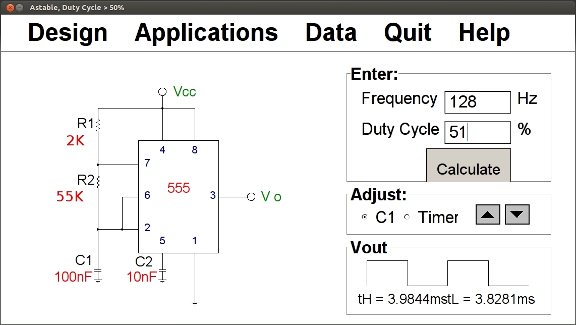
Figure 47 : 555 timer schematic.
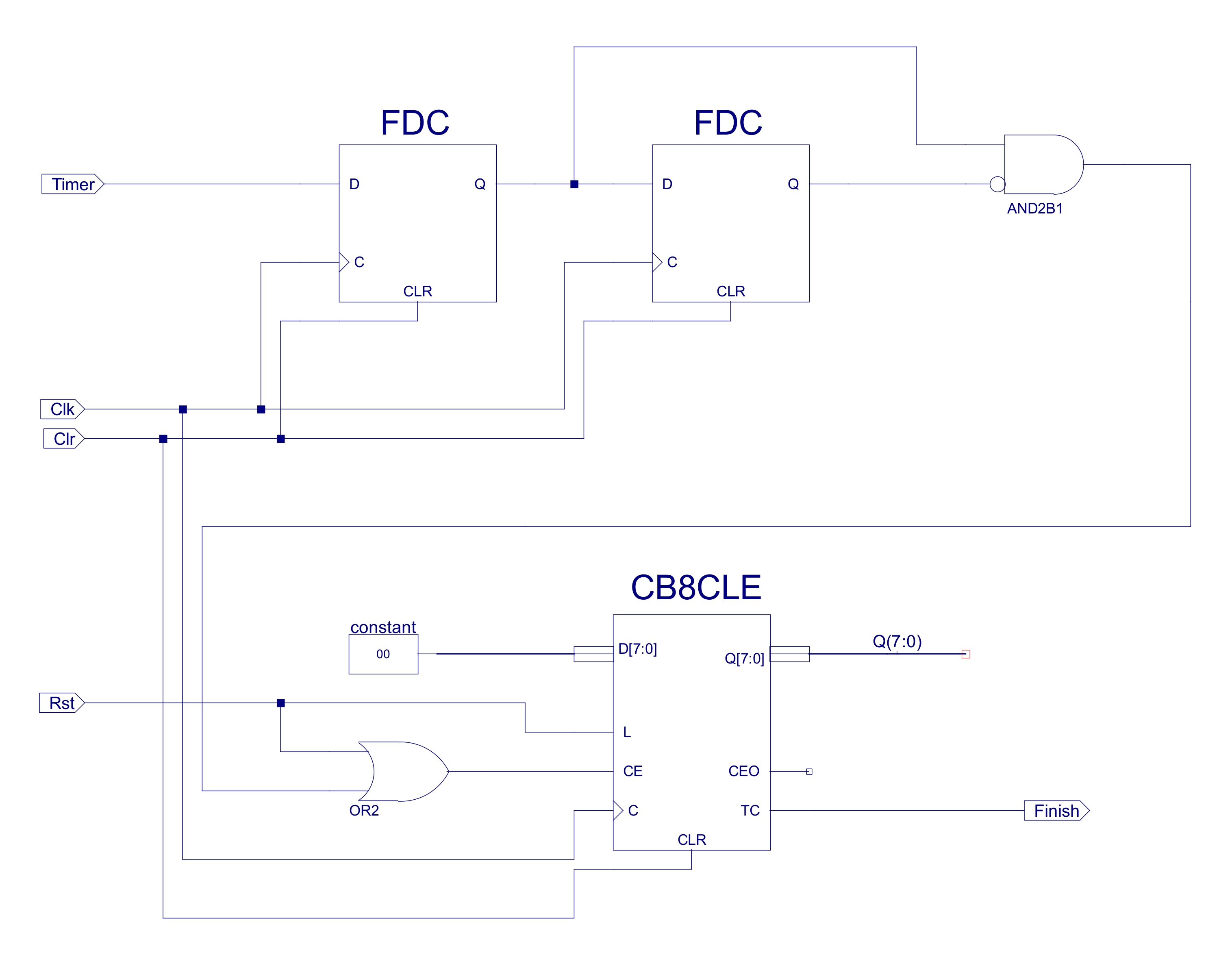
Figure 48 : 555 timer controller schematic.

Figure 49 : Explore hardware usage.
Bumper (whisker) sensors are implemented using simple switches, as shown in figure 50. Ideally i would passed these signals through an 74HC14 Schmitt triggers (Link) to 'square' these signals up a little more and help reduce glitches, but as space is limited used normal NOT gates on the CPLD. The manual reset (CLR) circuit is also shown. This uses a simple RC time delay to produce a power-on reset signal. The main system clock is provided by an 4MHz oscillator module: SG-615 (Link).
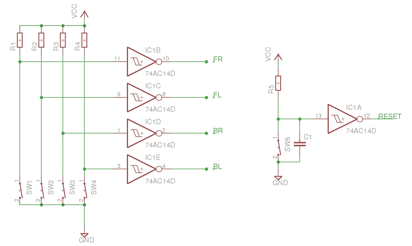
Figure 50 : Bumper switches and reset circuit.
To test the system's explore behaviours the series of test benches below were used.
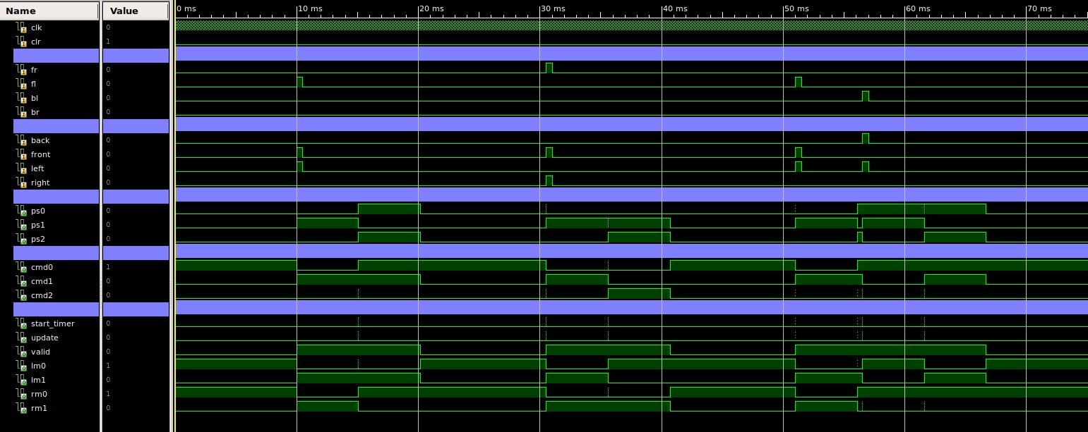
Figure 51 : Explore obstacle avoidance simulation.

Figure 52 : Explore looping simulation.

Figure 53 : Explore blocked-in simulation.
A lot bigger than i would liked (the final version will be cockroach sized), but this is what i had to hand: an old chassis and motor controller board from the first year DACS module, two CPLD modules and some blue boards, as shown in figure 54. Borrowed a 11V Lithium Polymer battery, mounting it over one wheel is not the best idea, as it will make the robot even more unlikely to travel in a straight line, but space was limited. Opposite this is the power regulator board, a couple of 7805 (Link) to convert the battery voltage down to a +5V, one for the logic and one for the motors. Again, if i had the choice would replace these linear regulators with switch mode versions, dumping 6V across these regulators means they get a little warm, also wasting power which doesn't do much for battery life.

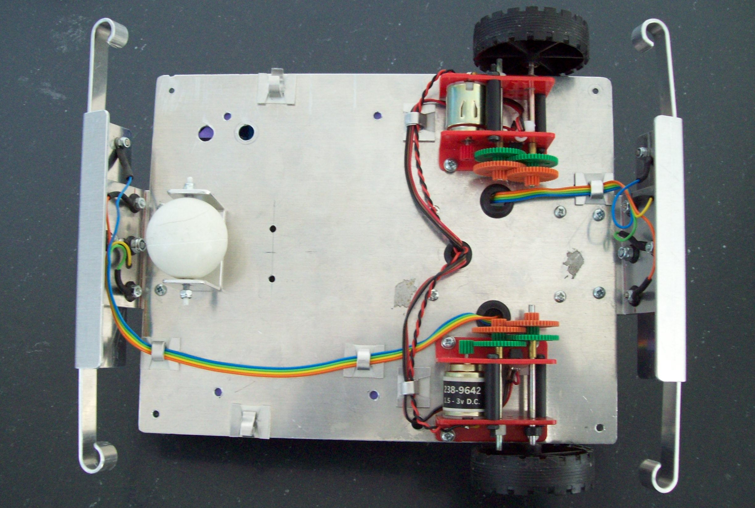
Figure 54 : Prototype 1
The motor controller board and analogue interface schematics and PCB are shown in figures 55 - 58.
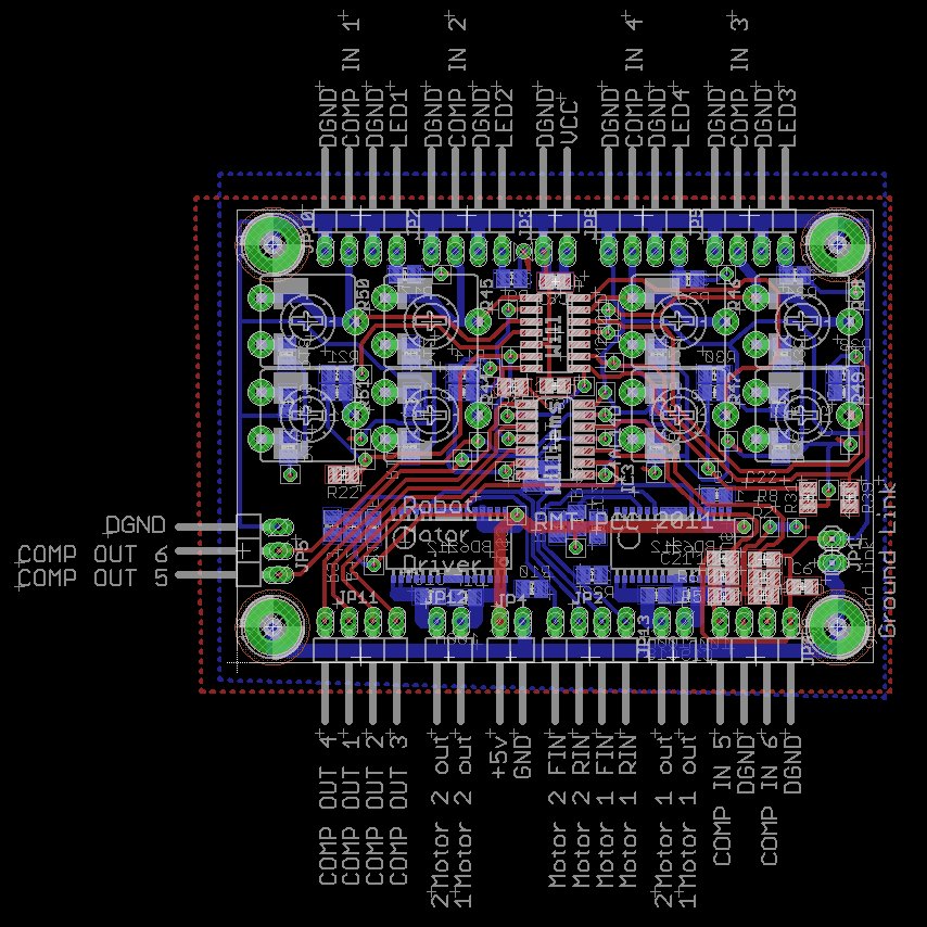
Figure 55 : Motor controller + analogue interface PCB
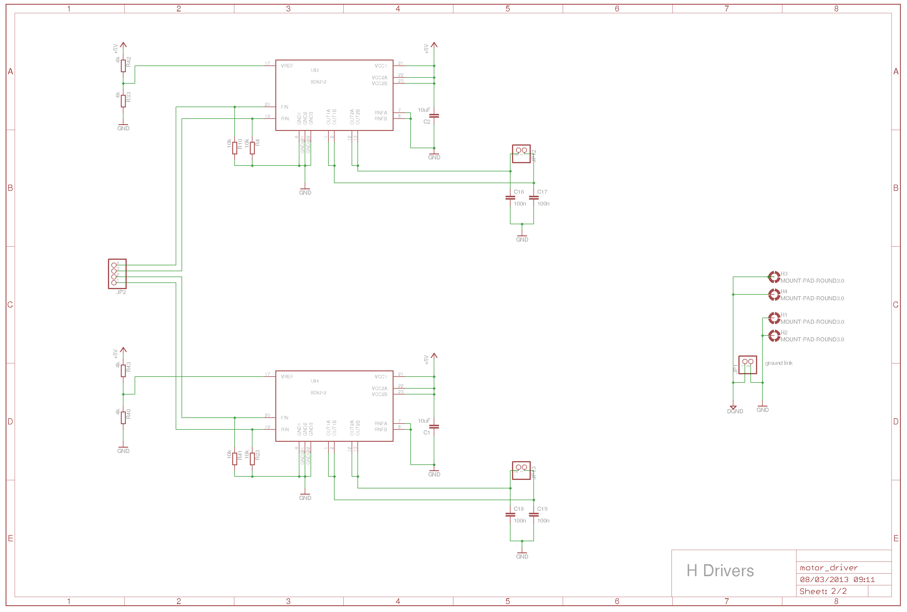
Figure 56 : H-bridge motor controllers
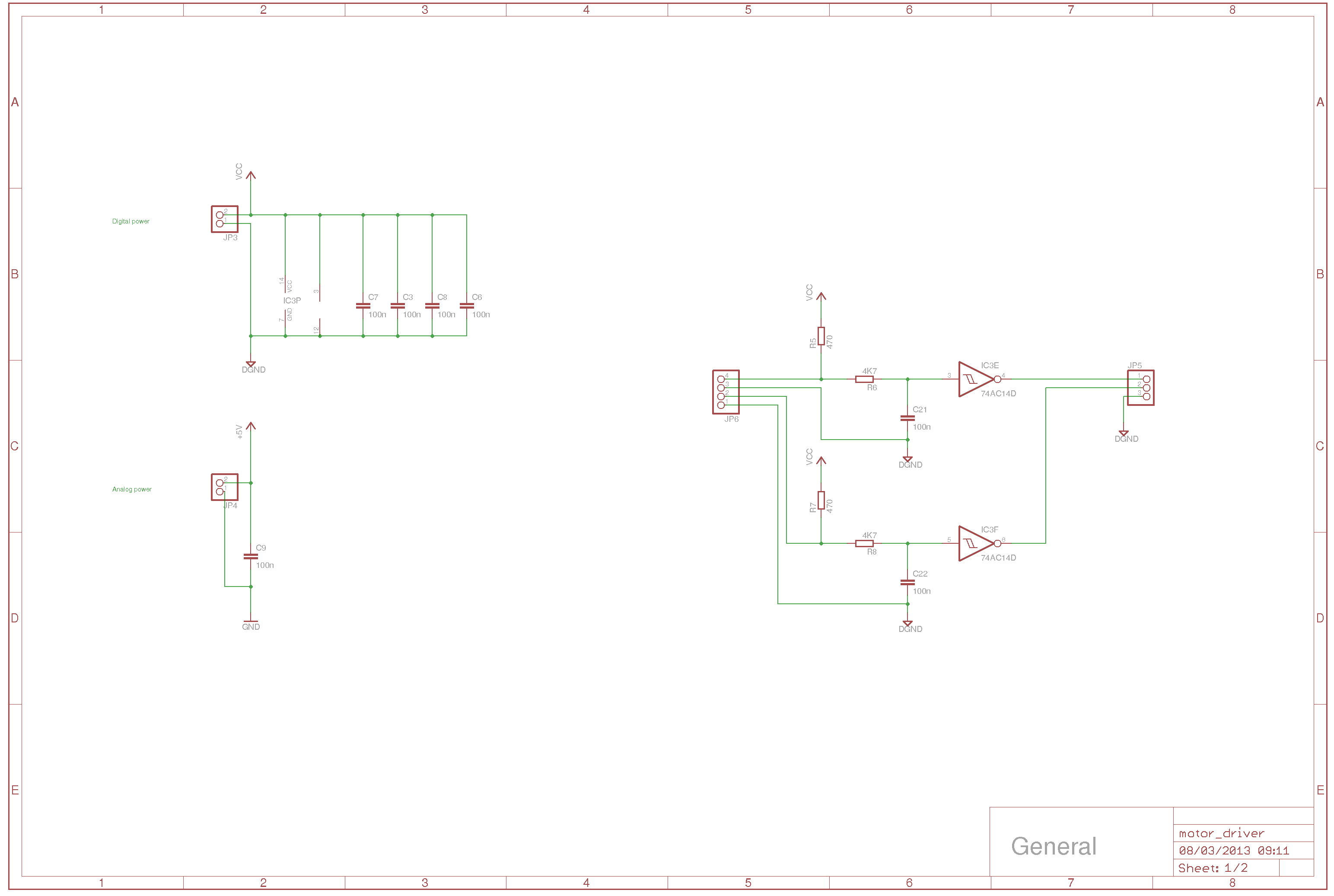
Figure 57 : Switch de-bounce buffers
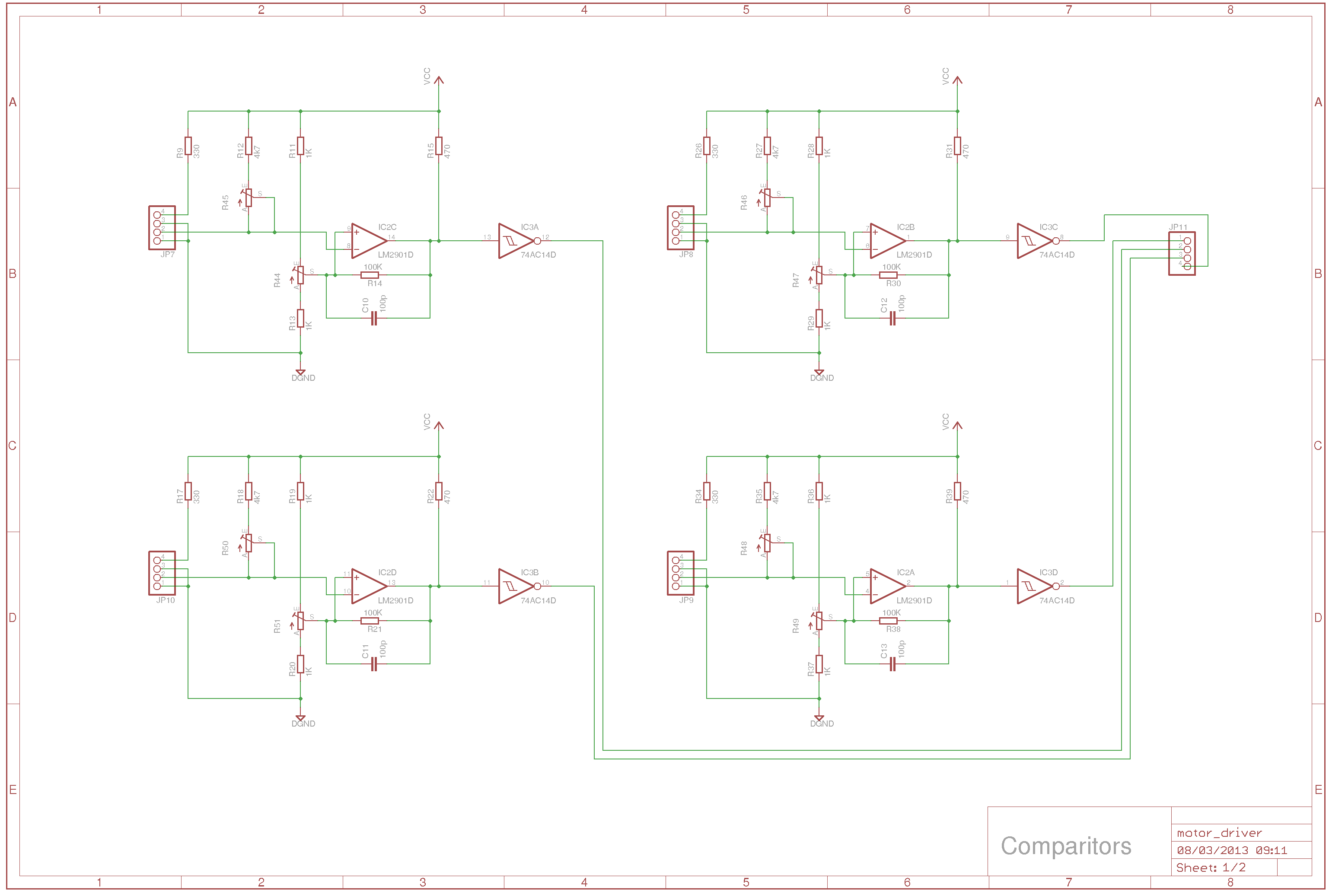
Figure 58 : analogue Schmitt trigger buffers
Below is a list of the main external connections to the CPLD. Note, the picture in figure 54 has two CPLDs, just in case the final solution needs more than the 72 macro cells (flip-flops) available.
System wiring:
Bumper wiring:
Motor control wiring:
Made a few videos of the robot in action, showing its explore, looping and block-in behaviours. Seems to work ok, there are a few false movements owing to switch bounce i.e. when the robot hits an obstacle you can get multiple transition on the bumper signals, which will confuse the state machines. Should be relatively simple to remove out using either analogue low pass filters (LPF), or another state machines i.e. hardware that makes sure the signal is stable before passing it on to the other state machines. These switching problems should not come as a surprise when you look at the actual switches, shown in figure 58. The front plate is wired to 0V (blue wire), this is held in place with an M4 bolt. The other switch contacts are also M4 bolts (connected to the orange, yellow and green wires) mounted in rubber grommets to insulate then from the chassis / front plate. When assembled if the robot bumps into an obstacle the front plate is pushed onto one or more of these bolts, completing the circuit. This allows the robot to sense the location of an obstacle as: middle, left or right (middle contact not used at the moment).
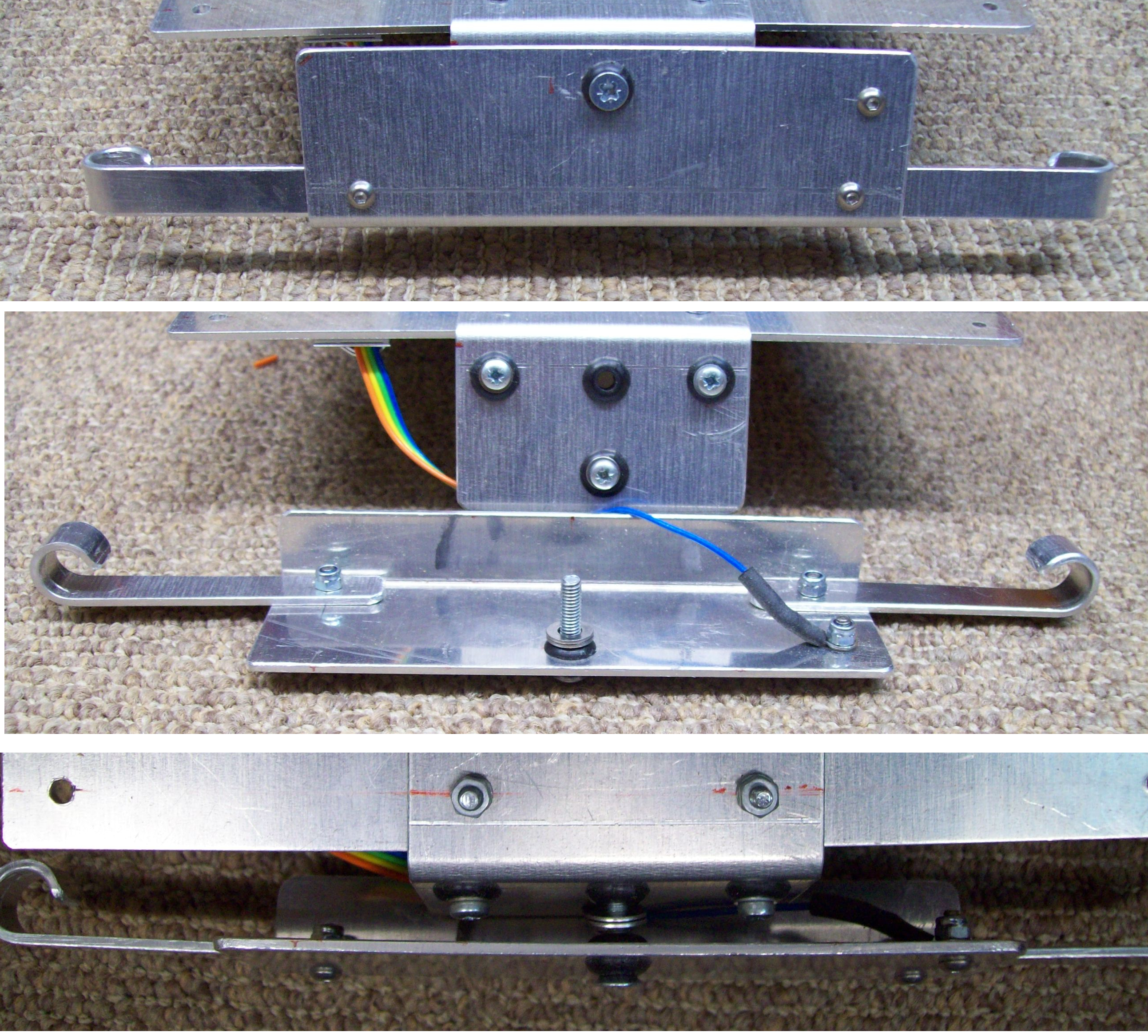
Figure 59 : Bumper switches
Phase two. The first set of state machines are complete, its now time to add some additional sensors. Most cockroaches prefer dark places, or only come out at night. A simple sensor to measure the environments illumination levels is a Light Dependent Resistor (LDR) i.e. a resistor who's resistance is inversely proportional to light levels (Link). This can be used in a simple potential divider circuit, producing a voltage that is inversely proportional to the background light level i.e. 0V = bright, +5V = dark. Interfacing this voltage to the digital system would normally require an Analogue to Digital Converter (ADC), however, as space is limited i'm going to go for a 1bit ADC i.e. a NOT gate. This digital logic gate defines a range of voltages for a logic '0' and a logic '1'. Therefore, with careful selection of the potential divider resistors the NOT gate can be used to produce a very simple (bad) analogue to digital output i.e. 0=dark, 1=bright. Note, to allow adjustments i used a 470 fixed in series with 10K variable for the top resistor. Using this signal a state machine can be designed to move the robot away from bright lights i.e. rotate 180 degrees and move in the opposite direction.
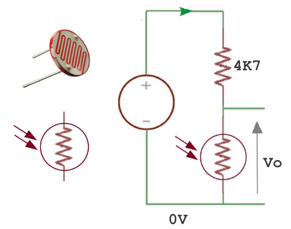
Figure 60 : LDR sensor (top left), symbol (bottom left), potential divider circuit (right)
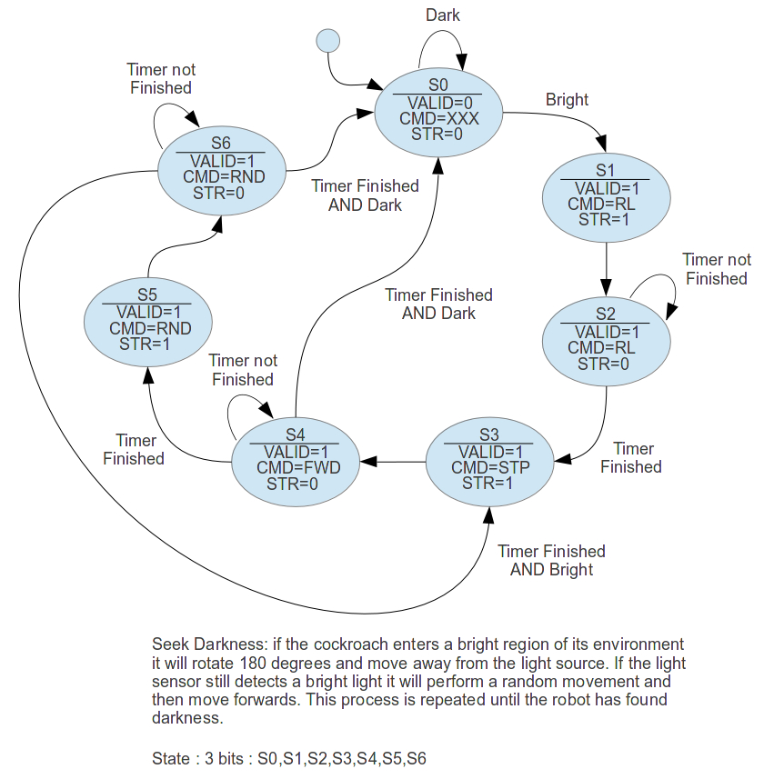
Figure 61 : Avoid light state machine
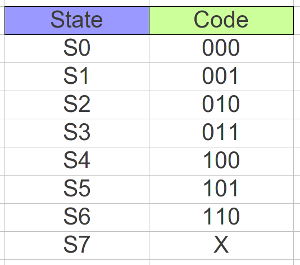
Figure 62 : Avoid light state encoding.
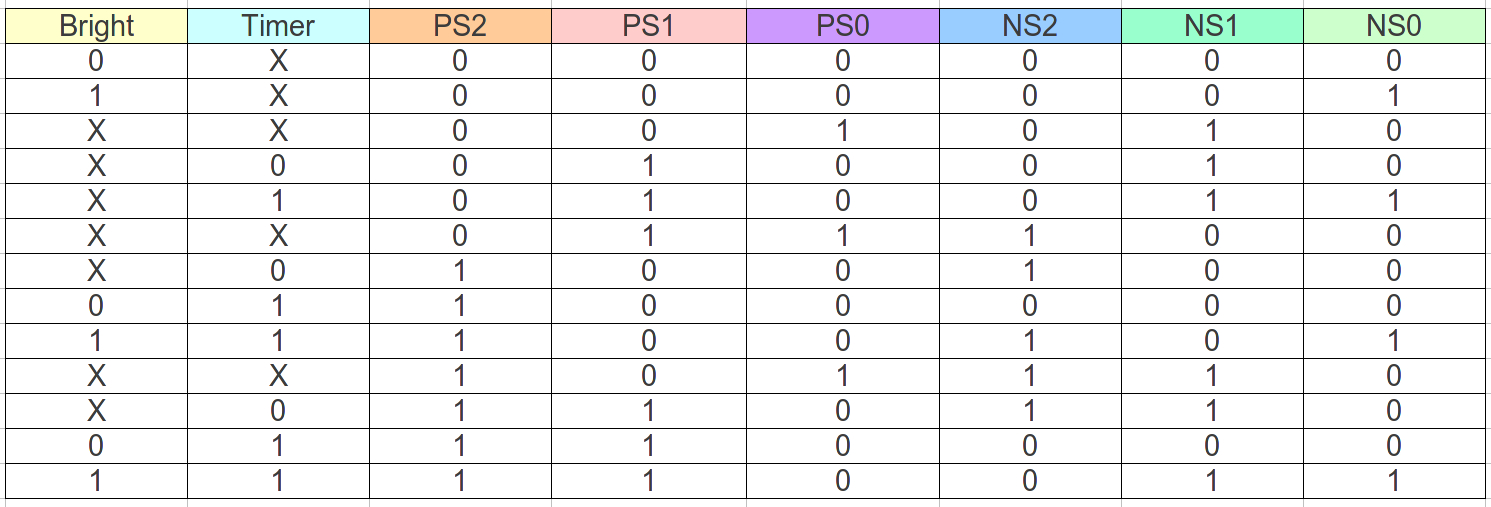
Figure 63 : Avoid light input forming logic.
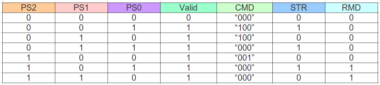
Figure 64 : Avoid light output forming logic.
NS2 <=           ( Bright and not PS1 and     PS2)
              or (    PS0 and     PS1 and not PS2)
              or (    PS0 and not PS1 and     PS2)
              or (not PS0 and     PS2 and not Timer);

NS1 <=           ( Bright and not PS0 and     PS1)
              or (    PS0 and not PS1)
              or (not PS0 and     PS1 and not PS2)
              or (not PS0 and     PS1 and not Timer);

NS0 <=           (Bright and not PS0 and     Timer)
              or (Bright and not PS0 and not PS1 and not PS2)
              or (           not PS0 and     PS1 and not PS2 and Timer);

Valid <=         (    PS0 and not PS1)
              or (    PS1 and not PS2)
              or (not PS0 and     PS2);

random <=        (    PS0 and not PS1 and PS2)
              or (not PS0 and     PS1 and PS2);

start_timer <=   (PS0 and not PS1)
              or (PS0 and not PS2);

CMD2 <=          (    PS0 and not PS1 and not PS2)
              or (not PS0 and     PS1 and not PS2);

CMD1 <=       '0';

CMD0 <=          (not PS0 and not PS1 and PS2);
Figure 65 : Minimised logic equations
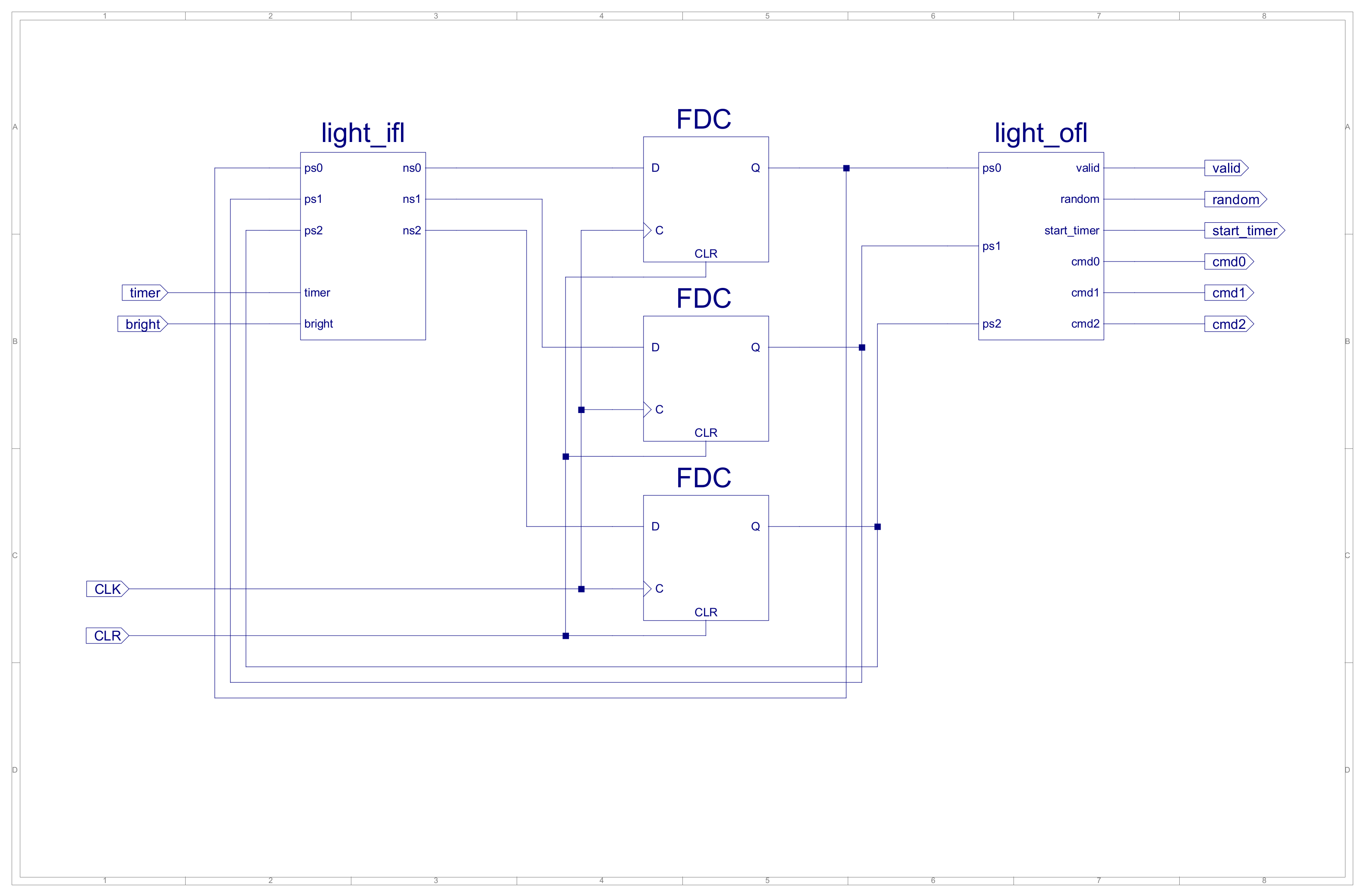
Figure 66 : Avoid light schematic.
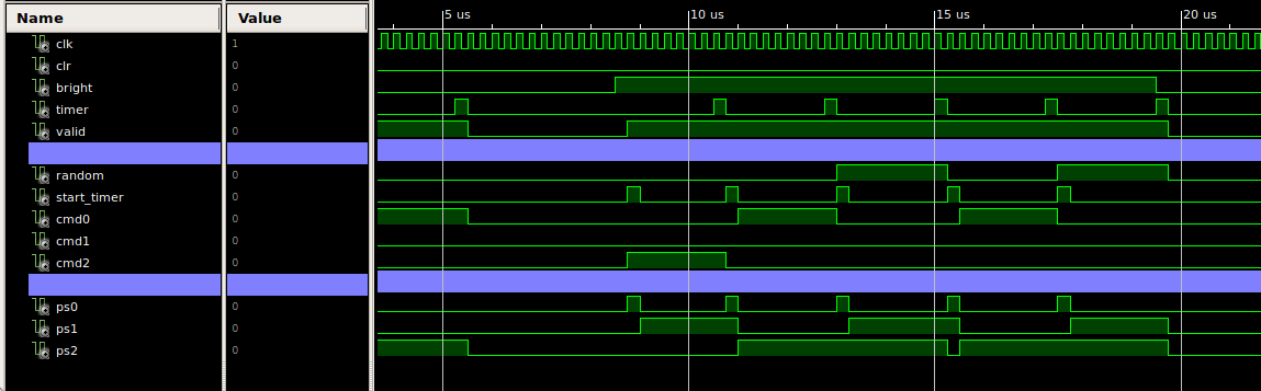
Figure 67 : Avoid light simulation.
In the previous state machines a 2 second delay was sufficient to turn the robot away from an obstacle, however, in the Light state machine i need a longer time delay. Therefore, added an additional 4 bit counter to the existing 8 bit counter, as shown in figure 68. Here the Clock Enable Out (CEO) signal is used to enable the 4 bit counter i.e. it is only enabled when the 8 bit count has reached its maximum count value (255). The outputs of the 4 bit counter are then decoded using AND gates to produce an output pulse when each of its outputs goes to a logic '1' for the first time. Note, each output of the 4 bit counter effectively doubles the time delay.
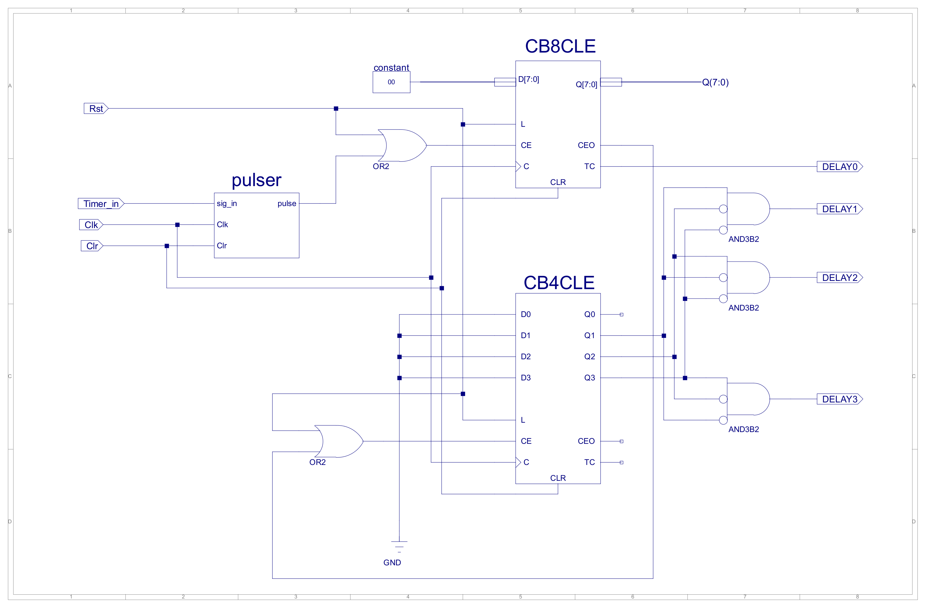
Figure 68 : Delay timer.
When the robot encounters a bright area it will turn around and move back the way it has come, however, if the background illumination level of its environment should increase e.g. the change from night to morning, the robot will need to seek a dark place to hide. To implement this behaviour the robot will perform a random movement followed by a move forwards until it finds a dark place. In the previous state machine a random movement was implemented using a free running counter. This 'random' value was generated owing to the high frequency of the clock used compared to the random nature / timing of when the robot would bump into an obstacle. This technique will not work for the Light state machine as the timing is fixed by the hardware i.e. counter will always count to the same value. To add a little more variability a Linear Feedback Shift Register (LFSR) circuit is used, as shown in figure 69 and 71. A description can be found here: (Link). This circuit is commonly used as a random number generator. Again this circuit does not generate a truly random value, but it does generate a sequence of values that give the illusion of randomness. The output of the LFSR is then decoded using a logic circuit to produce the desired three bit movement command. To save time this has been implemented in VHDL as shown in figure 72. The CPLD software tools then automatically synthesize this into the logic circuit show in figure 73. To be honest, using a LFSR may not be the best solution, it may be more efficient in terms of hardware to use a 3bit counter and a ROM 8x3bit containing a predefined list of movements i.e. a lookup table defining a search pattern.
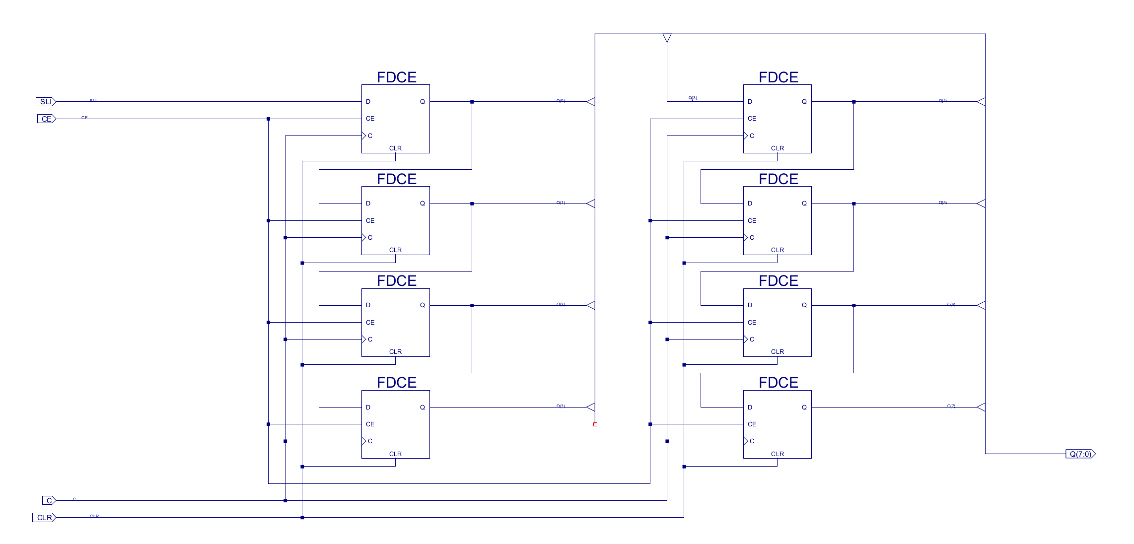
Figure 69 : SR8CE, 8bit shift register.
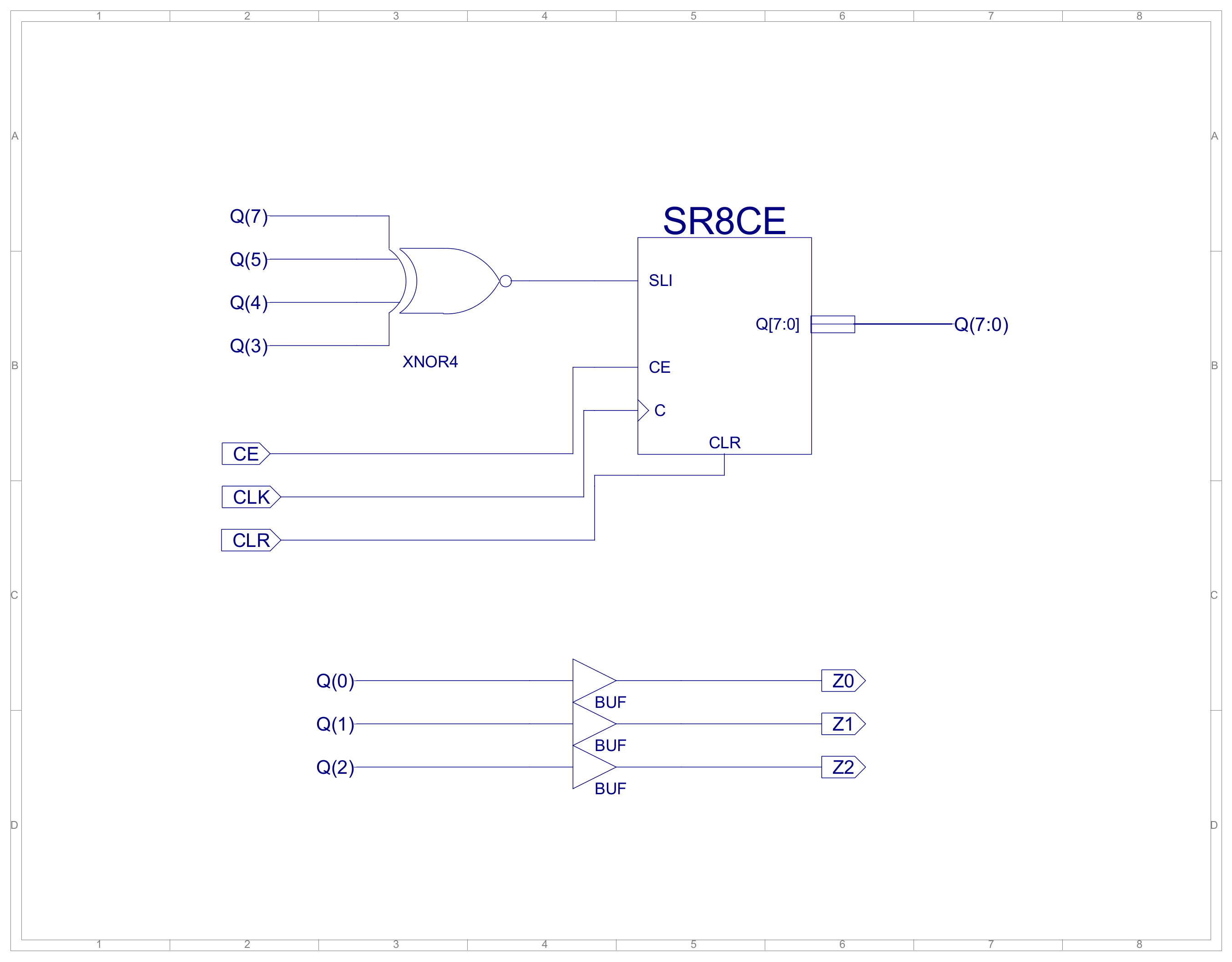
Figure 70 : LFSR.
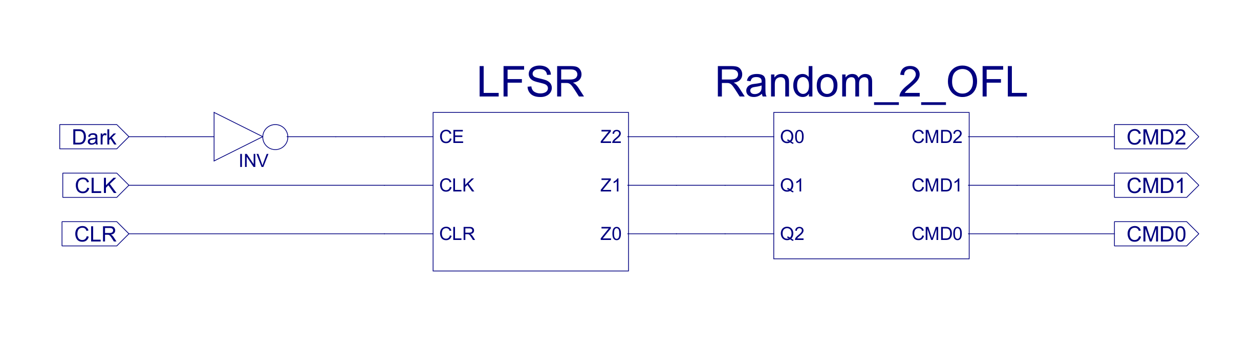
Figure 71 : Random movement command.
library IEEE;
use IEEE.STD_LOGIC_1164.ALL;

entity Random_2_OFL is
    Port ( Q0   : in  STD_LOGIC;
           Q1   : in  STD_LOGIC;
           Q2   : in  STD_LOGIC;
           CMD2 : out STD_LOGIC;
           CMD1 : out STD_LOGIC;
           CMD0 : out STD_LOGIC );
end Random_2_OFL;

architecture Random_2_OFL_arch of Random_2_OFL is

	constant STOP         : std_logic_vector(2 downto 0) := "000";
	constant FORWARDS     : std_logic_vector(2 downto 0) := "001";
	constant BACKWARDS    : std_logic_vector(2 downto 0) := "010";
	constant ROTATE_RIGHT : std_logic_vector(2 downto 0) := "011";
	constant ROTATE_LEFT  : std_logic_vector(2 downto 0) := "100";
	constant TURN_RIGHT   : std_logic_vector(2 downto 0) := "101";
	constant TURN_LEFT    : std_logic_vector(2 downto 0) := "110";
	constant BREAK        : std_logic_vector(2 downto 0) := "111";

	signal Count   : std_logic_vector(2 downto 0);
	signal Command : std_logic_vector(2 downto 0);

begin

   Count <= Q2 & Q1 & Q0;
   CMD2  <= Command(2);
   CMD1  <= Command(1);
   CMD0  <= Command(0);

   logic: process( Count )
   begin
      case Count is
         when "000"  => Command <= ROTATE_RIGHT;
         when "001"  => Command <= ROTATE_LEFT;
         when "010"  => Command <= TURN_RIGHT;
         when "011"  => Command <= BACKWARDS;
         when "100"  => Command <= ROTATE_LEFT;
         when "101"  => Command <= FORWARDS;
         when "110"  => Command <= TURN_LEFT;
         when "111"  => Command <= ROTATE_LEFT;
         when Others => Command <= STOP;
      end case;
   end process;

end Random_2_OFL_arch;
Figure 72 : Random movement logic.
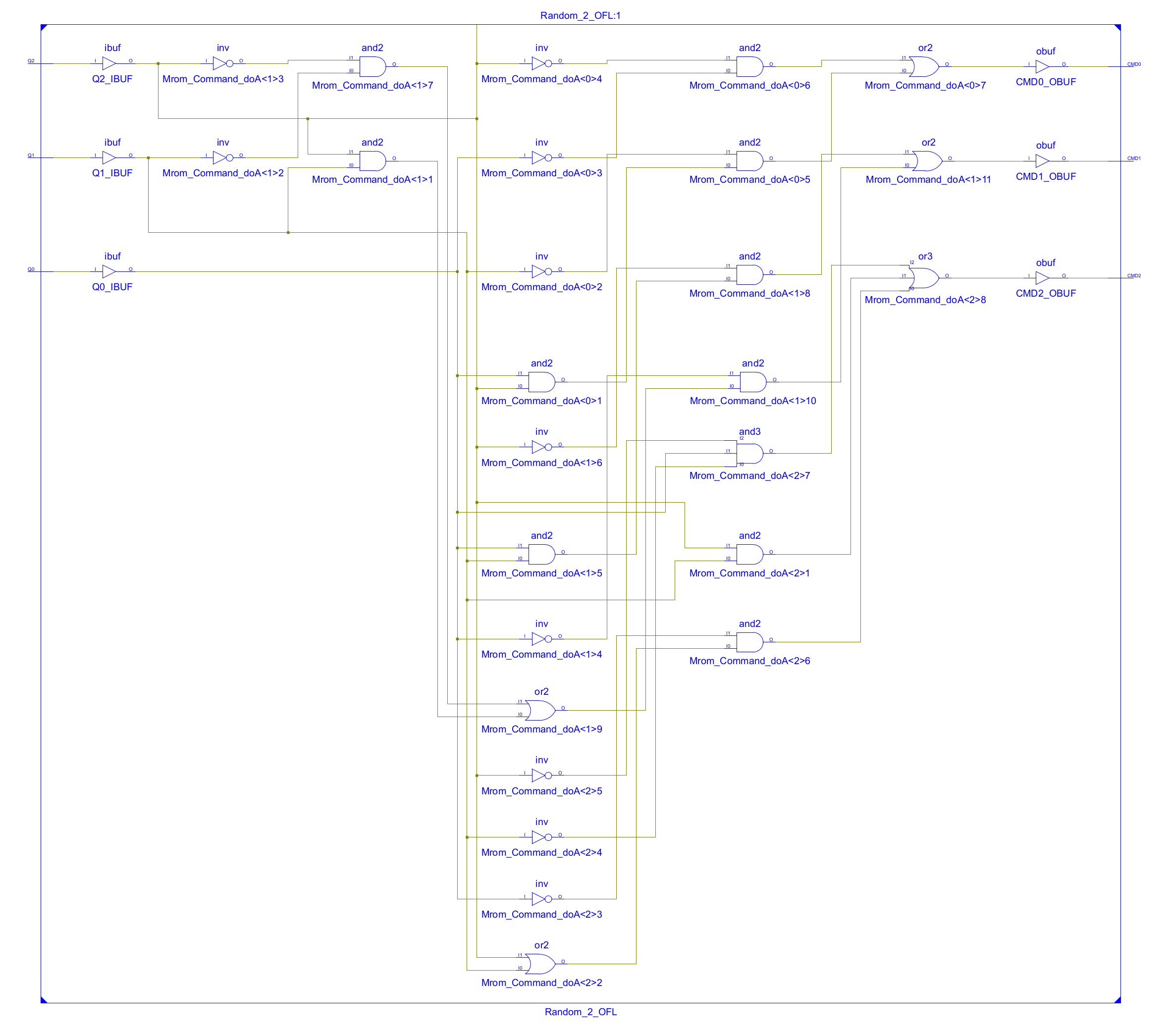
Figure 73 : Random movement logic.
In addition to the LDR sensor the robot also has a tilt sensor, as shown in figure 74. This is constructed from a simple pendulum (bolt + nut) and a loop of wire, each forming the contacts of a switches. When the robot goes up a slope i.e. from underground, up into the light, the switch contacts will be made. In this situation the desired behaviour will be the same as the Light sensor i.e. turn around and go back the way it came. Therefore, the Light sensor and the Tilt sensor can be used to trigger the same state machine. To prevent sudden direction changes generating false tilt sensor readings the output of this signal is passed through a low pass filter, as shown in figure 75 i.e. fast changing signals are blocked, or to think about it another way it now takes a significant period of time to change up the voltage on the capacitor to a logic '1'.
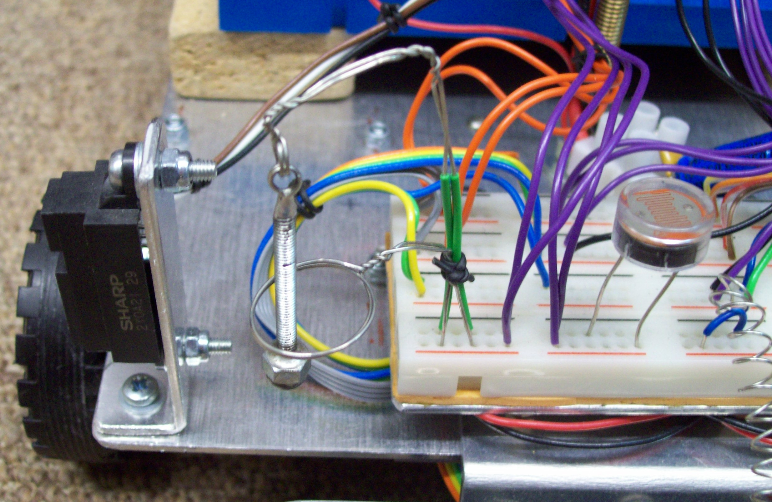
Figure 74 : Sensors: distance (left), tilt (middle), light (right)
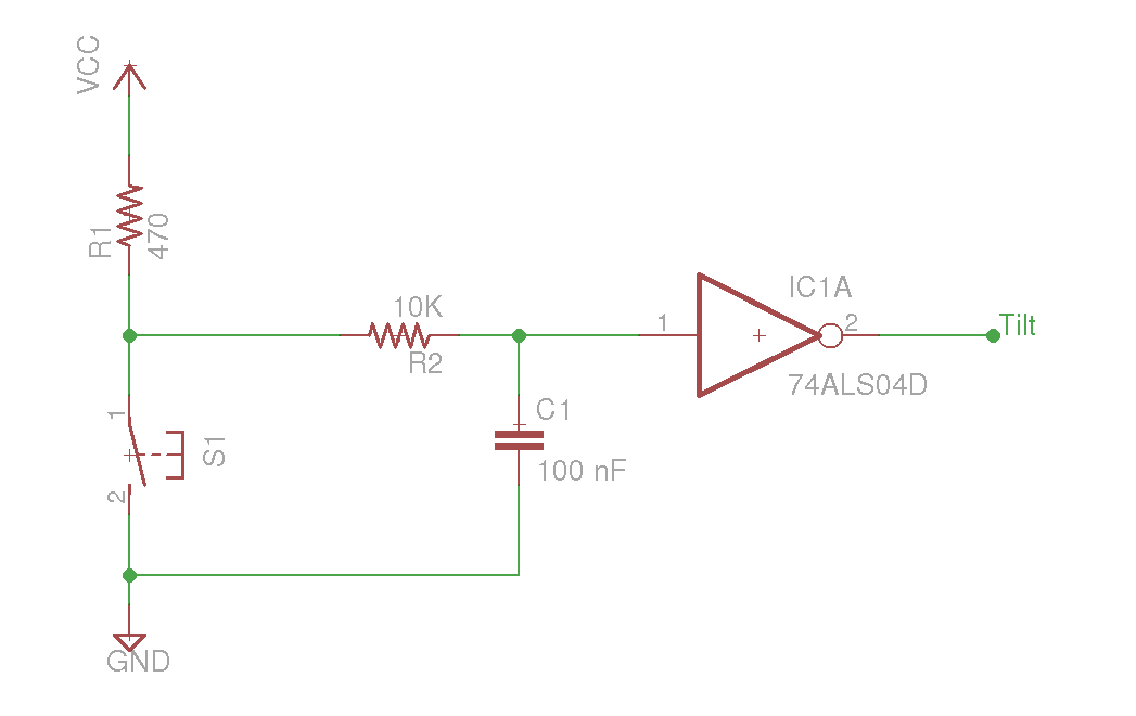
Figure 75 : Tilt sensor low pass filter.
Made a few videos of the robot in action, move back into the dark works ok, but find dark doesn't, turning 180 degrees doesn't allow the robot to really explore its environment i.e. it moves back over the same ground, need to vary the delay i.e. turn 90 degrees.
To alter the cockroach's behaviour need to redesign the input forming logic, as shown in figure 76. There are now two timer inputs: long and short. Also altered the output forming logic so that the default command for state 0 was move forwards rather than don't care, as shown in figure 77. The complete Light behaviour test system circuit diagram is shown in figure 78 (the Light state machine now has two timer inputs).
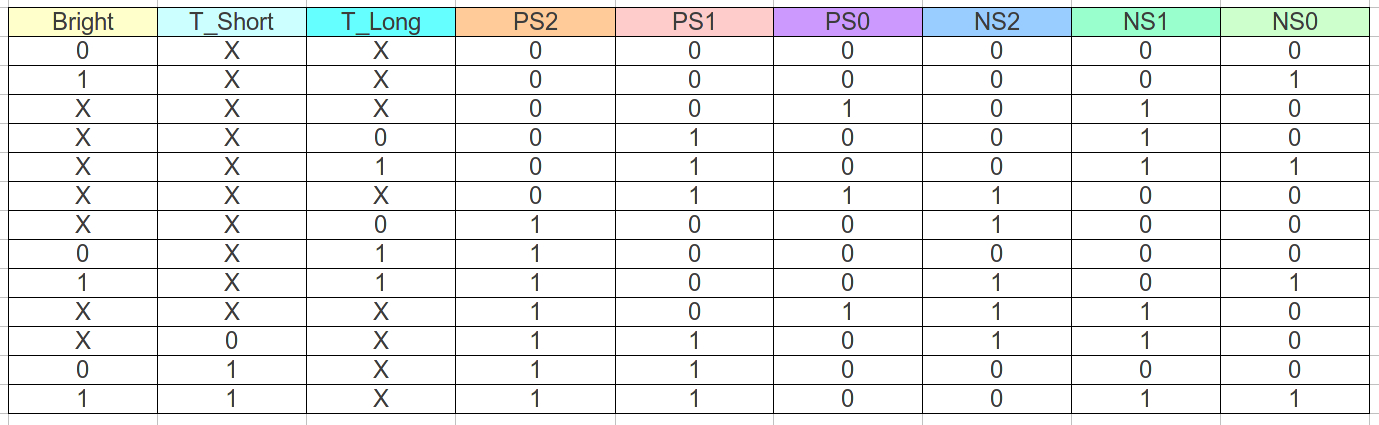
Figure 76 : New Light input forming logic truth table.
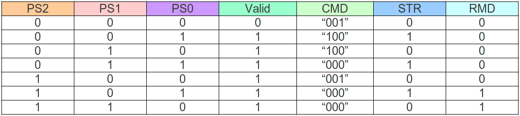
Figure 77 : New Light output form logic truth table.
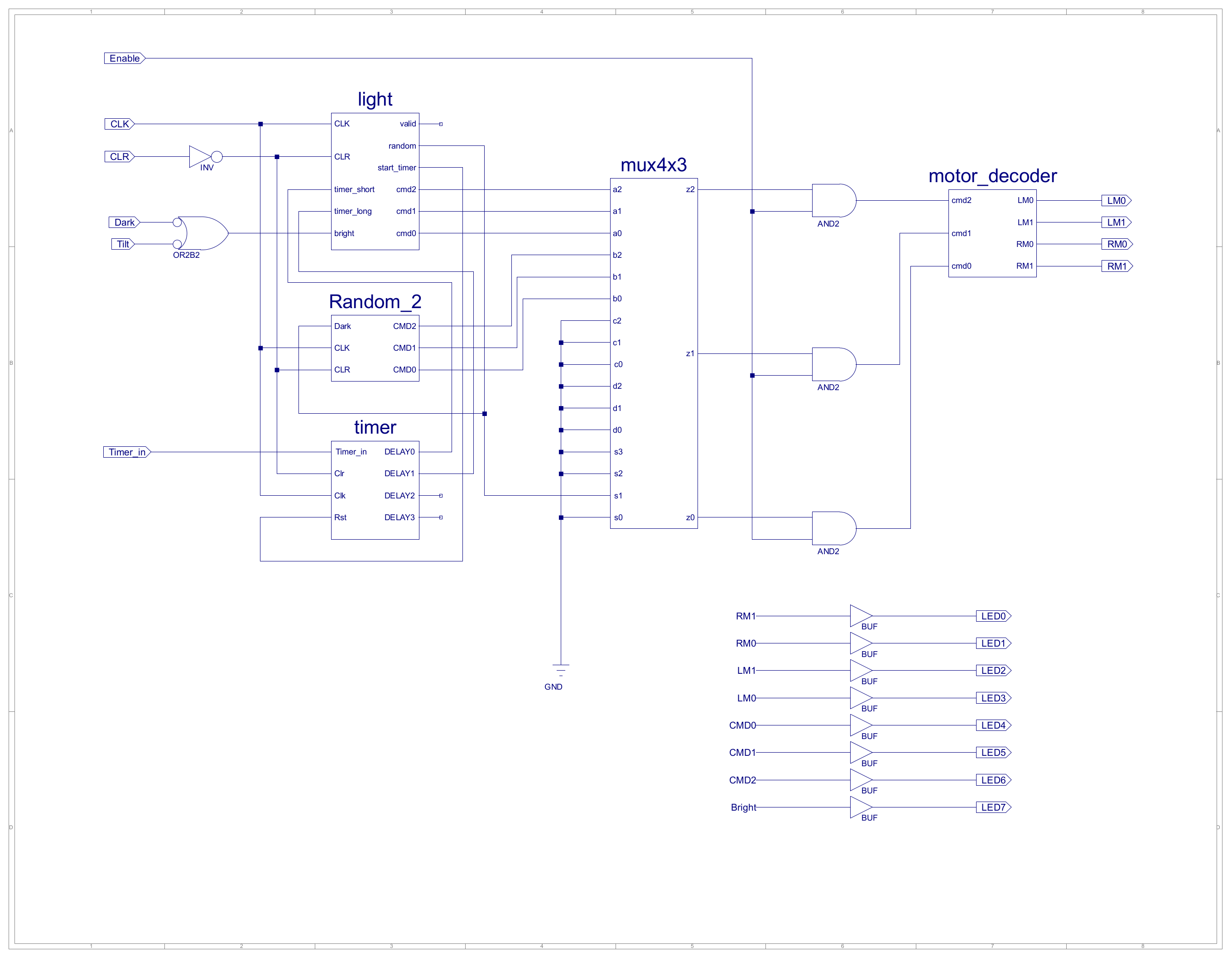
Figure 78 : Light test system
To improve the cockroaches explore behaviour distance sensors can be mounted on the chassis, allowing the robot to measure the distance to obstacles in its environment, as shown in figure 79. This sensor is a Sharp GP2Y0A21 general purpose infra-red distance sensor (Link), producing an analogue voltage that is inversely proportional to distance. Again, like the seek dark behaviour looking for a simple solution, ideally based on a single sensor. Subsumption architecture behaviours should be simple and fast, the wall following behaviour may not work in all situations, or be the most complete, however, the interaction of the different state machines shown in figure 4 should give the desired cockroach like behaviour. The state diagram for the wall following behaviour is shown in figure 80.
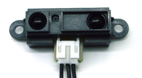
Figure 79: Sharp infra-red distance sensor
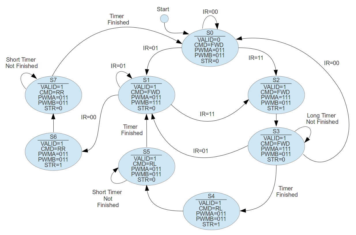
Figure 80: Wall following state diagram
The analogue signal from the sensor is passed to two analogue comparators as shown in figure 58 (four in schematic). An analogue comparator is based around an operational amplifier (Link) and compares an unknown voltage (infra-red sensor) to a reference voltage (potential divider, variable resistor on PCB). For this particular implementation if the sensor signal is greater than the reference voltage it will output a logic '1'. The sensor's voltage output response is shown in figure 81, setting these reference voltages to 1V and 2V allows the robot to detect obstacles at approximately 25cm and 15cm, producing a two bit output:
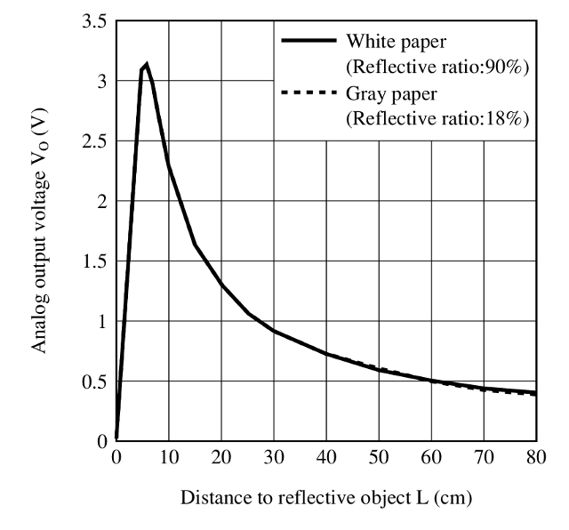
Figure 81: Infra-red sensor signal
When the cockroach does not detect an object (code 00) it uses its explore behaviour to move. The infra-red sensor is mounted on the cockroach's right hand side, when it detects a distant object (code 01) it increases the speed of the left motor, slowly turning the robot towards the object. If it then detects that it is too close (code 11), it reduces the speed of the left motor and increases the speed of the right motor to move away from the obstacle. Therefore, if the cockroach does find a wall the robot flips between these two behaviours, maintaining a 'fixed' distance to the wall. This behaviour is modified by states S3 and S6. If the cockroach is unable to turn away from the wall sufficiently quickly (long time out signal), it will perform a quick rotate left command to move away from the wall. If the cockroach has lost the wall it will perform a quick rotate right command to point the cockroach back towards the 'wall'. Made a short video of the cockroach in action, to prevent it looping will need the loop detector:
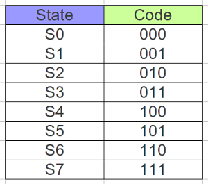
Figure 82: Wall following state encoding
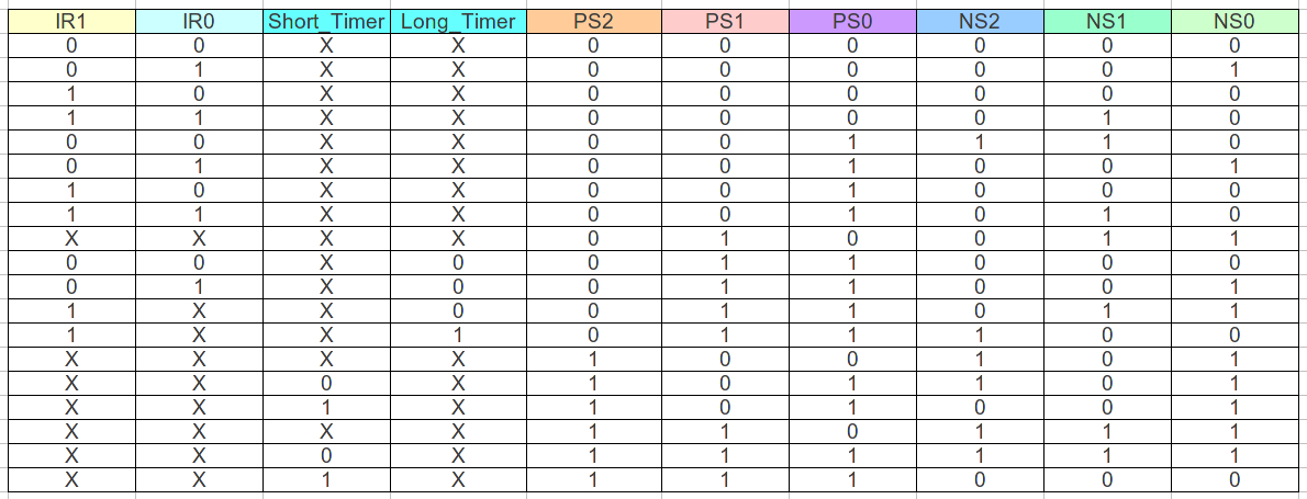
Figure 83: Wall following input forming logic truth table
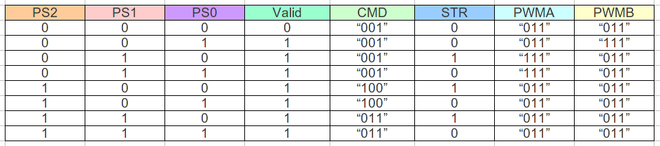
Figure 84: Wall following output forming logic truth table
NS2 <=       (IR1 and     Long_Timer and     PS0 and     PS1 and not PS2)
      or     (PS2 and not Short_Timer)
      or (not IR0 and not IR1        and     PS0 and not PS1 and not PS2)
      or (not PS0 and     PS2);


NS1 <=       (IR0 and     IR1        and not PS1         and not PS2)
      or     (IR1 and not Long_Timer and     PS1         and not PS2)
      or     (PS1 and     PS2        and not Short_Timer)
      or (not IR0 and not IR1        and     PS0         and not PS1 and not PS2)
      or (not PS0 and     PS1);

NS0 <=       (IR0 and not IR1        and not PS1)
      or     (IR0 and not Long_Timer and     PS1 and not PS2)
      or     (IR1 and not Long_Timer and     PS1 and not PS2)
      or     (PS2 and not Short_Timer)
      or (not PS0 and     PS1)
      or (not PS1 and     PS2);

Valid       <= not PS2 and not PS1 and not PS0;

CMD2        <= not PS1 and     PS2;
CMD1        <=     PS1 and     PS2;
CMD0        <=     PS1 or  not PS2;

Start_Timer <= (not PS0 and PS1) or (not PS0 and PS2);

PWMA        <=     PS1 and not PS2;
PWMB        <=     PS0 and not PS1 and not PS2;
Figure 85 : Wall following IFL and OFL
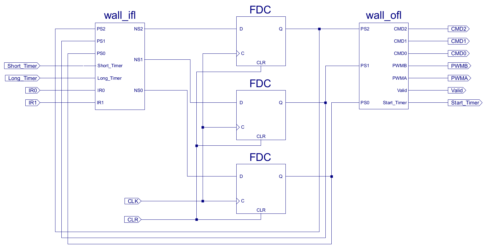
Figure 86: Wall following state machine
command <= cmd2 & cmd1 & cmd0;

logic : process( command )
begin
    case command is
        when "000"  => LM1 <= '0'; LM0 <= '0'; RM1 <= '0'; RM0 <= '0'; --stop
        when "001"  =>
            if pwma = '1'
            then
                LM1 <= '0'; LM0 <= '1'; RM1 <= '0'; RM0 <= pwm;	--forward fast lm
            elsif pwmb = '1'
            then
                LM1 <= '0'; LM0 <= pwm; RM1 <= '0'; RM0 <= '1';	--forward fast rm
            else
                LM1 <= '0'; LM0 <= pwm; RM1 <= '0'; RM0 <= pwm;	--forward slow
            end if;
        when "010"  =>
            if pwma = '1'
            then
                LM1 <= '1'; LM0 <= '0'; RM1 <= pwm; RM0 <= '0';	--back fast lm
            elsif pwmb = '1'
            then
                LM1 <= pwm; LM0 <= '0'; RM1 <= '1'; RM0 <= '0';	--back fast rm
             else
                LM1 <= pwm; LM0 <= '0'; RM1 <= pwm; RM0 <= '0';	--back slow
             end if;
        when "011"  => LM1 <= '1'; LM0 <= '0'; RM1 <= '0'; RM0 <= '1';	--rotate right
        when "100"  => LM1 <= '0'; LM0 <= '1'; RM1 <= '1'; RM0 <= '0'; --rotate left
        when "101"  => LM1 <= '0'; LM0 <= '1'; RM1 <= '0'; RM0 <= '0';	--turn right
        when "110"  => LM1 <= '0'; LM0 <= '0'; RM1 <= '0'; RM0 <= '1'; --turn left
        when "111"  => LM1 <= '1'; LM0 <= '1'; RM1 <= '1'; RM0 <= '1';	--brake
        when others => LM1 <= '0'; LM0 <= '0'; RM1 <= '0'; RM0 <= '0';	--stop
    end case;
end process;
Figure 87 : Wall following motor control logic
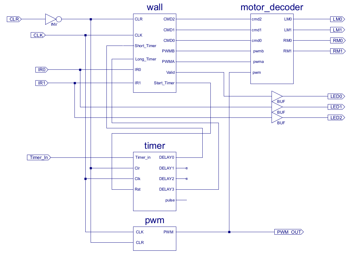
Figure 88: Wall following top level
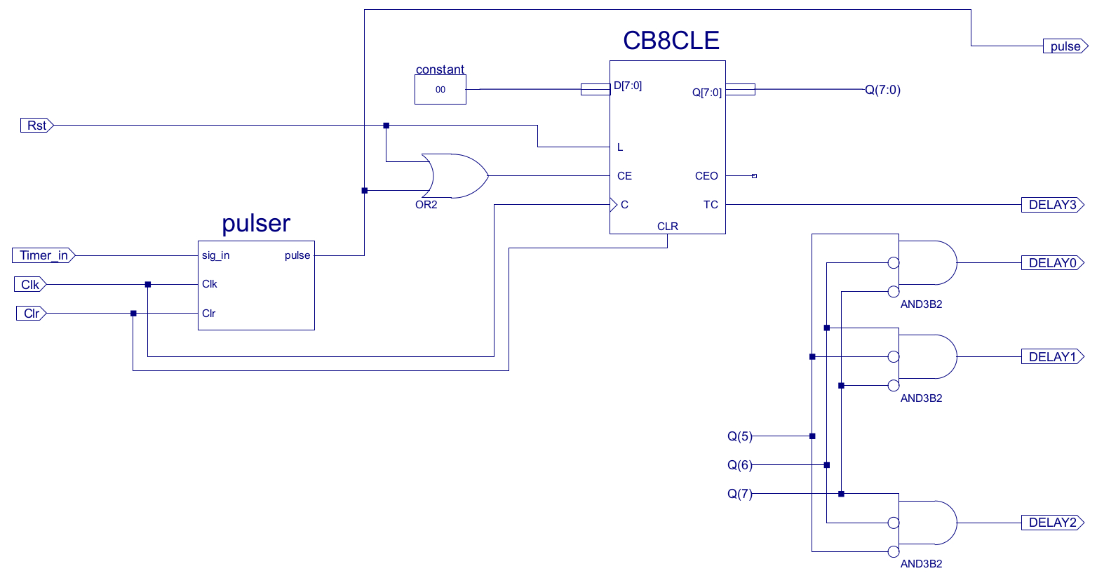
Figure 89: Wall following timer
To control the speed of the motors a techniques called pulse width modulation (PWM) is used, as shown in figure 90. By altering the ratio of the voltage ON / OFF time, the speed of the motor can be varied. A simple analogy would be pressing, then releasing the accelerator in a car i.e. the ratio of powered drive to coasting, if this done fast enough it will give the illusion of driving at a slower speed. From an electrical point of view this approach minimises power lost in the drive transistors, the DC drive motors can be considered to be a resistor (R) and inductor (L) in series, these will store electrical energy during the ON time, then smooth out the flow of current in the OFF time i.e. act as a low pass filter. The PWM waveform is generated by the circuit shown in figure 91. The frequency of this waveform must be fast enough to avoid a "jittery" motor response, but not too fast to be completely filtered out by the motor. Therefore, the CB16CE counter is used to divide down the 4MHz system clock. This is then passed through an edge detector, which in turn is used to enable a ring counter. The six stage ring counter is loaded with the pattern "111100" i.e. 4/6 motor power, which is logical ANDed with the motor to control logic i.e. the motor will drive forwards for 4/6 of the time and coast for 2/6 of the time. To increase motor speed the motor drive logic is set to a constant logic '1' i.e. equivalent to a PWM pattern of "111111" i.e. drive forwards 6/6 of the time, full motor power. To be honest this solution is a little complex, could achieve the same result with a simple counter, may redesign later.
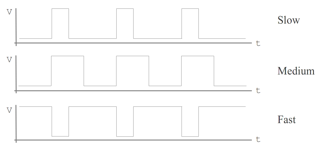
Figure 90: Pulse width modulation
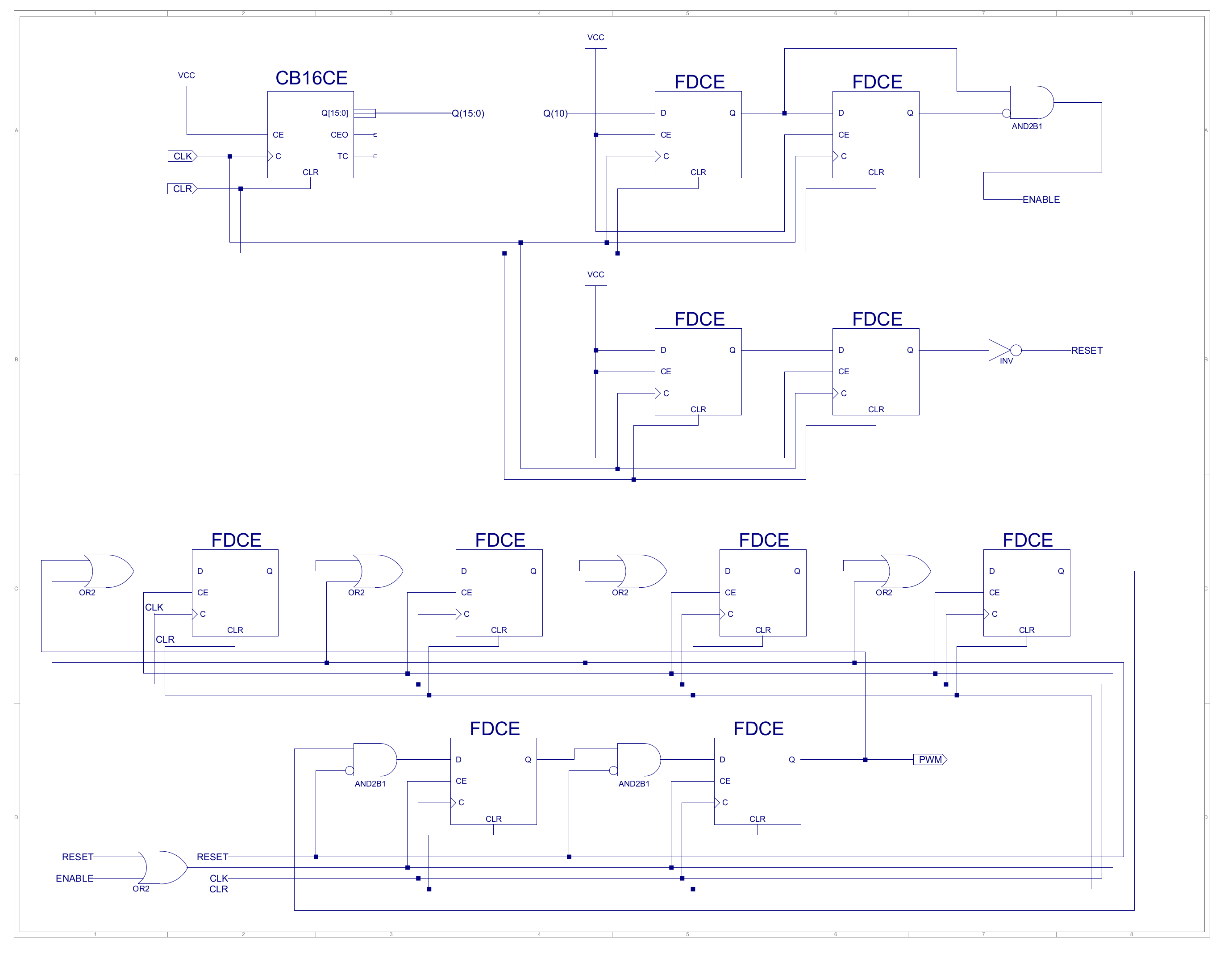
Figure 91: Wall following motor speed control
Food for the cockroach is electrical power. Therefore, the robot will have two probes (mouth parts) that trail on the ground 'tasting' for food. Food are disks of aluminium foil, as shown in figure 92. These are wired to a +12V power supply
With two or more LDR sensors mounted in a linear array the cockroach can implement a slightly more intelligent control system. Using two LDR sensors on the front of the cockroach it can measure the difference between the light levels on the left and right hand side. The difference between these signals indicates which way the cockroach should turn in order to avoid the light. To allow the robot to gradually adjust its trajectory the speed of each drive motor needs to be controlled e.g. increasing the speed of the drive motor on the brighter side of the robot will cause it to veer away from the light. To control the speed of a motor Pulse Width Modulation (PWM) can be used, as shown in figure 70.
This is as far as i got with this robot, would of liked to have got a smaller more polished final version working as an open day demo i.e. a group of cockroaches in an constrained environment, interacting with each other, exploring, searching for food etc, would be interesting to watch / identify more complex behaviours develop. One day :(. If anyone would like to make their own version of this robot the Xilinx ISE project files can be downloaded here: (Link)

This work is licensed under a Creative Commons Attribution-NonCommercial-NoDerivatives 4.0 International License.
Contact details: email - mike.freeman@york.ac.uk, telephone - 01904 32(5473)
Back